12  Software

12.1 Software Overview

The Marine Sensitivity Toolkit (MST) is a stack of software components for reproducibly, interactively and hierarchically generating environmental vulnerability maps and scores. Tabular data is collated across studies evaluating sensitivity of species to oil & gas and offshore wind energy development. The best available species and benthic habitat distributions are being mosaicked across the US EEZ. Scores are summarized according to subgroups within Species, Benthic Habitats and Primary Productivity, averaged into an overall score, and visualized as a flower plot, applicable to various levels of BOEM relevancy: regional, ecoregions, protraction diagrams, blocks and aliquots.

The software components for achieving this interactively are:

1. server — a Docker Compose configuration orchestrating the reverse proxy, Shiny server, APIs, TiTiler raster serving and file server;
2. database — a columnar, embedded analytic database (DuckDB) as the single source of truth for species distributions, per-cell scores and derived per-zone metrics;
3. workflows — Quarto notebooks to ingest source datasets (AquaMaps, IUCN, NMFS/FWS, BirdLife, WoRMS, BOEM zones), merge taxonomic authorities, and compute scores that are written back to DuckDB;
4. APIs — a custom R plumber API for data requests, TiTiler serving the published COGs, and a searchable STAC API with one Item per model;
5. libraries — re-usable documented functions as the msens R package, including the version/manifest registry that lets one application render any release, and the tile-URL helpers the applications use;
6. applications — two Shiny apps (scores, species) that combine COG raster layers with static PMTiles vector layers and live-pushed choropleth paint rules, each rendering any published release from ?ver=;
7. documentation — this Quarto book with figures, tables, glossary and references in interactive HTML or static DOCX / PDF output.

This toolbox is intended to primarily serve BOEM needs internally, but by being open-source and fully reproducible the hope is to enlist buy-in and even contributions from external partners, whether from other government agencies, academia, NGOs or industry.

We ascribe to the philosophy of sharing all code for the sake of reproducibility, transparency and efficiency (Maitner et al. 2024; Lowndes et al. 2017); i.e. the FAIR principles of Findability, Accessibility, Interoperability, and Reusability (Wilkinson et al. 2016).

Figure 12.1: System architecture: a release is published as partitioned Parquet plus pre-rendered COGs. TiTiler serves the score rasters; zone polygons are served as static PMTiles through Caddy; the Shiny apps combine both layer types and push per-zone scores live into the polygon paint spec.

12.1.1 Interactive Applications

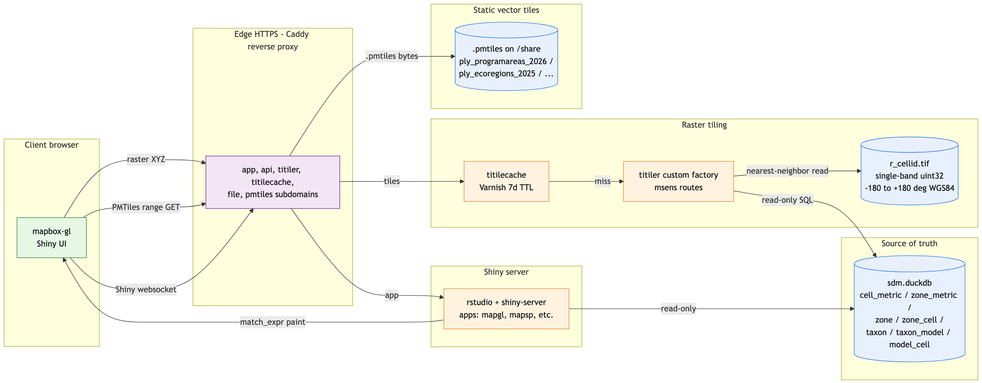
We have developed a series of interactive applications to explore the data and results of the MST project. These applications allow users to visualize the data, explore the results, and interact with the data in a more intuitive way. The applications are built using the shiny package in R (Chang et al. 2024), which allows us to easily create a user interface with complex reactivity for an interactive web application easily accessed through a web browser. The applications are designed to be user-friendly and intuitive, with interactive maps, charts, and tables that allow users to explore the data in a more dynamic way.

12.1.2 Overcoming Challenges with Large Spatial Data

The MST project incorporates many large spatial datasets that are problematic to render in a typical interactive application. For instance, the most common interactive mapping R package leaflet has a 4 MB limitation for displaying rasters (see “Large Raster Warning” in Raster Images • leaflet). Vectors (points, lines and polygons) get smoothed when containing many vertices, but contiguity between polygons is lost and rendering degrades depending on the user’s connection speed.

To work around these limitations we use a “cloud native” stack (see also the Cloud-Optimized Geospatial Formats Guide) that transfers only the pixels / features visible in the current viewport:

• Raster cell values are published as pre-rendered Cloud-Optimized GeoTIFFs and delivered as small 256×256 PNG tiles by TiTiler’s stock /cog routes, which range-read only the part of the COG a tile needs.
• Vector polygons (Program Areas, Ecoregions, Planning Areas, …) are served as static PMTiles archives by the Caddy file server — a single archive per layer, range-read by the browser.
• Choropleth values (per-Program-Area scores) are pushed live from DuckDB into the PMTiles paint spec via a mapbox-gl match expression, so geometry stays static but color updates as the user changes metric / subregion.

Let’s take a closer look at each.

12.1.2.1 Raster: pre-rendered COGs

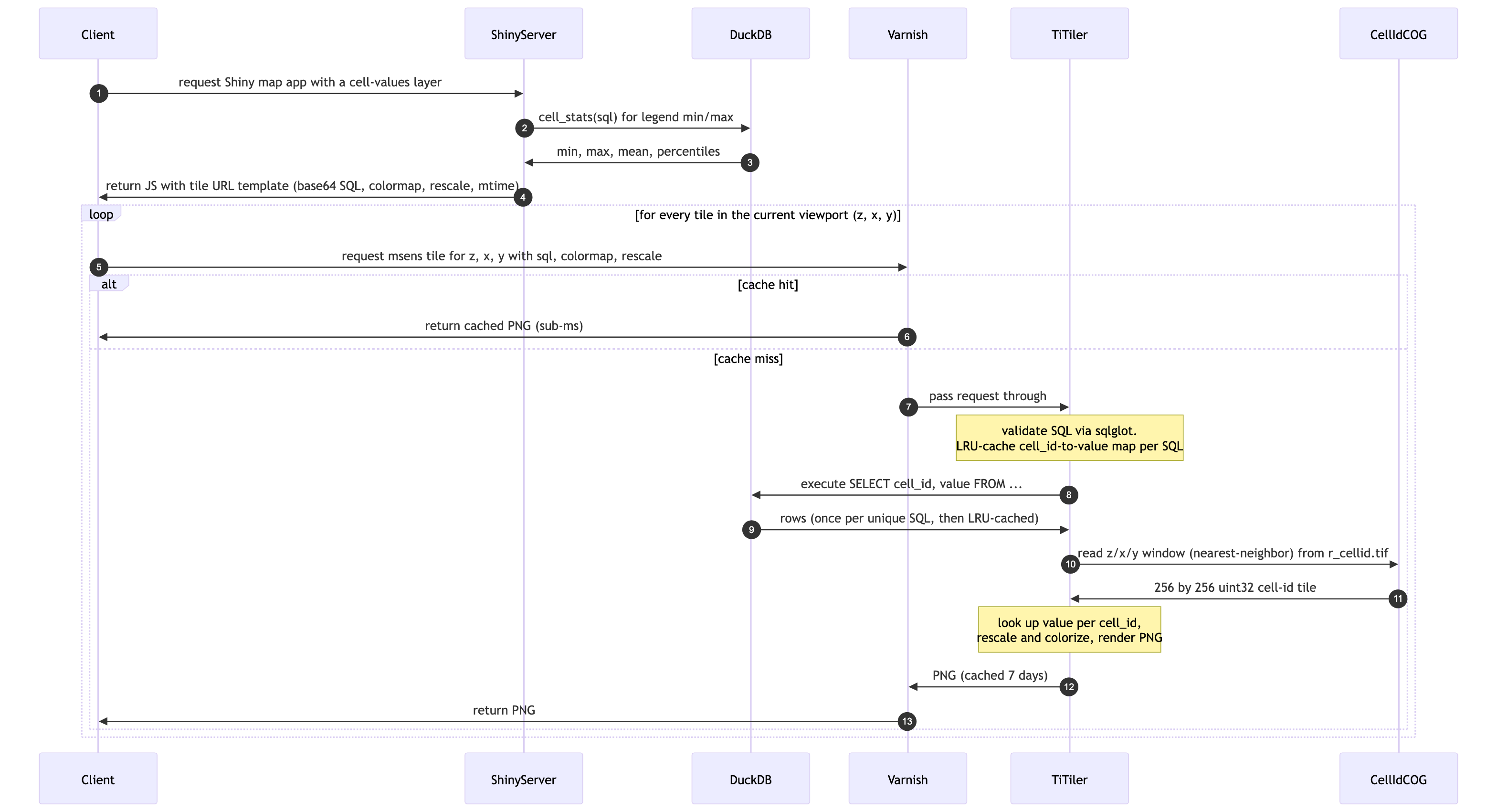
Each metric (e.g. extrisk_mammal) resolves, in DuckDB’s cell_metric table, to a list of (cell_id, val) rows — one per grid cell. Materializing the full raster and shipping it to the browser is not viable (several GiB), so only the tiles in view are transferred.

Scores are published as one COG per metric × subregion, written by a publishing workflow into a content-addressed store. Each release’s manifest carries the href and the build-time rescale range, so the application reads them and hands the URL to TiTiler’s stock /cog endpoints — no custom endpoint, and no database query in the tile path (Figure 12.2).

Two details are load-bearing:

• No overviews. The renderer decimates from full resolution on each request, so a pre-built pyramid would disagree with it at low zoom.
• The object key includes the encoding, not just the payload. Rewriting an object at a stable URL once left GDAL’s /vsicurl serving a cached header describing bytes that no longer existed: fine at z5+, HTTP 500 at z2–z4.

This replaced a custom TiTiler factory that rendered each tile by executing a validated SELECT against DuckDB and looking the result up against a pre-baked cell-id COG, with Varnish caching each tile URL for seven days. That path is retired but kept behind a flag (see Chapter 16); the two were verified to produce the same picture before the switch.

Figure 12.2: Sequence diagram: a cell-values raster layer is rendered on-the-fly by the custom msens TiTiler factory from the DuckDB source of truth. Varnish caches identical tile URLs for 7 days.

Binary overlays — the “cells outside Program Areas” mask — are published the same way, as their own single-color rasters rather than as a query.

12.1.2.2 Vector: static PMTiles served by Caddy

For polygon layers (Program Areas, Ecoregions, Planning Areas, protractions, blocks, aliquots) we build PMTiles archives offline via tippecanoe and publish them as static files on the server. A PMTiles archive is a single file with an internal directory structure that lets any HTTP client issue small range requests for individual tiles; no tile server process is required — Caddy’s static file handler is all we need (Figure 12.3).

Figure 12.3: Sequence diagram: vector layers are served as static PMTiles archives through Caddy. Each tile is a byte-range read of the archive — no tile server process is in the path.

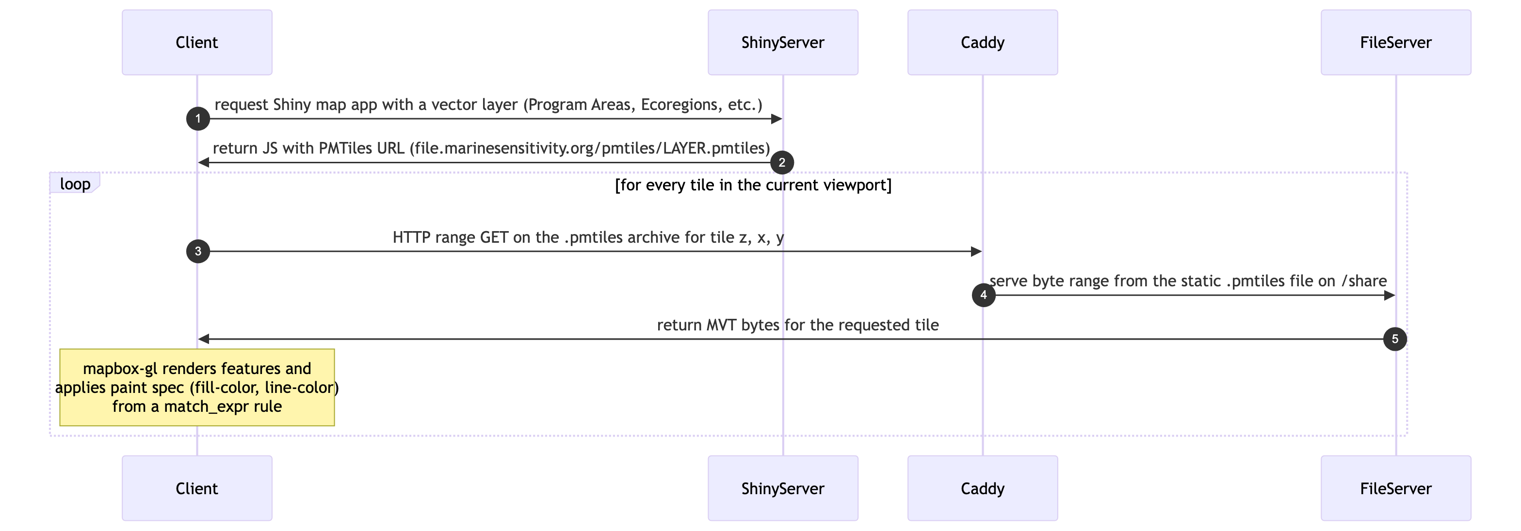
This is a deliberate simplification from the prior architecture which used PostgreSQL + PostGIS + pg_tileserv. For our workload — polygon layers that change only when the data is rebuilt — a compiled tile server and live database query engine add latency and operational complexity for no benefit over byte-range reads of a pre-baked archive. (PostgreSQL and pg_tileserv are now commented out of docker-compose.yml entirely and are not running; see Chapter 13.)

12.1.2.3 Choropleth: live DuckDB values + static PMTiles geometry

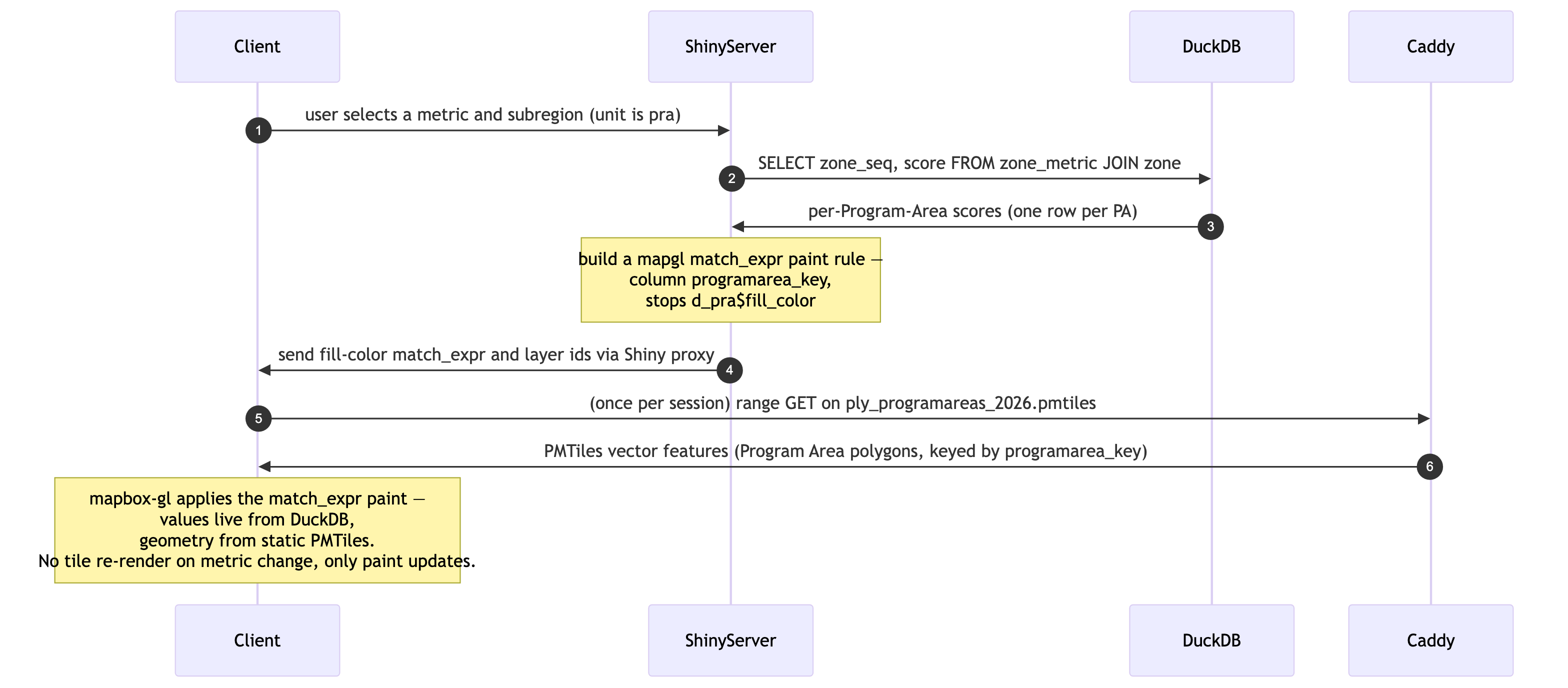
The Program Area choropleth is the interesting hybrid case. The geometry (Program Area polygons keyed by programarea_key) is static — it comes from the same PMTiles file as the polygon outlines. But the fill color depends on the currently-selected metric + subregion, which means the per-Program-Area score has to come live from DuckDB.

The Shiny server handles this by querying zone_metric (pre-aggregated per-zone values), building a mapbox-gl match expression that maps programarea_key → fill_color, and pushing that paint rule to the map through mapgl’s Shiny proxy. No tiles are re-rendered; only the paint specification changes (Figure 12.4).

Figure 12.4: Sequence diagram: the Program Area choropleth. Polygon geometry is static (PMTiles from Caddy file server); per-area fill values come live from DuckDB’s zone_metric table and are pushed into mapbox-gl’s paint spec via a match expression. Switching metrics updates only the paint rule, not the tiles.

12.1.2.4 Data pipeline — how the source of truth is built

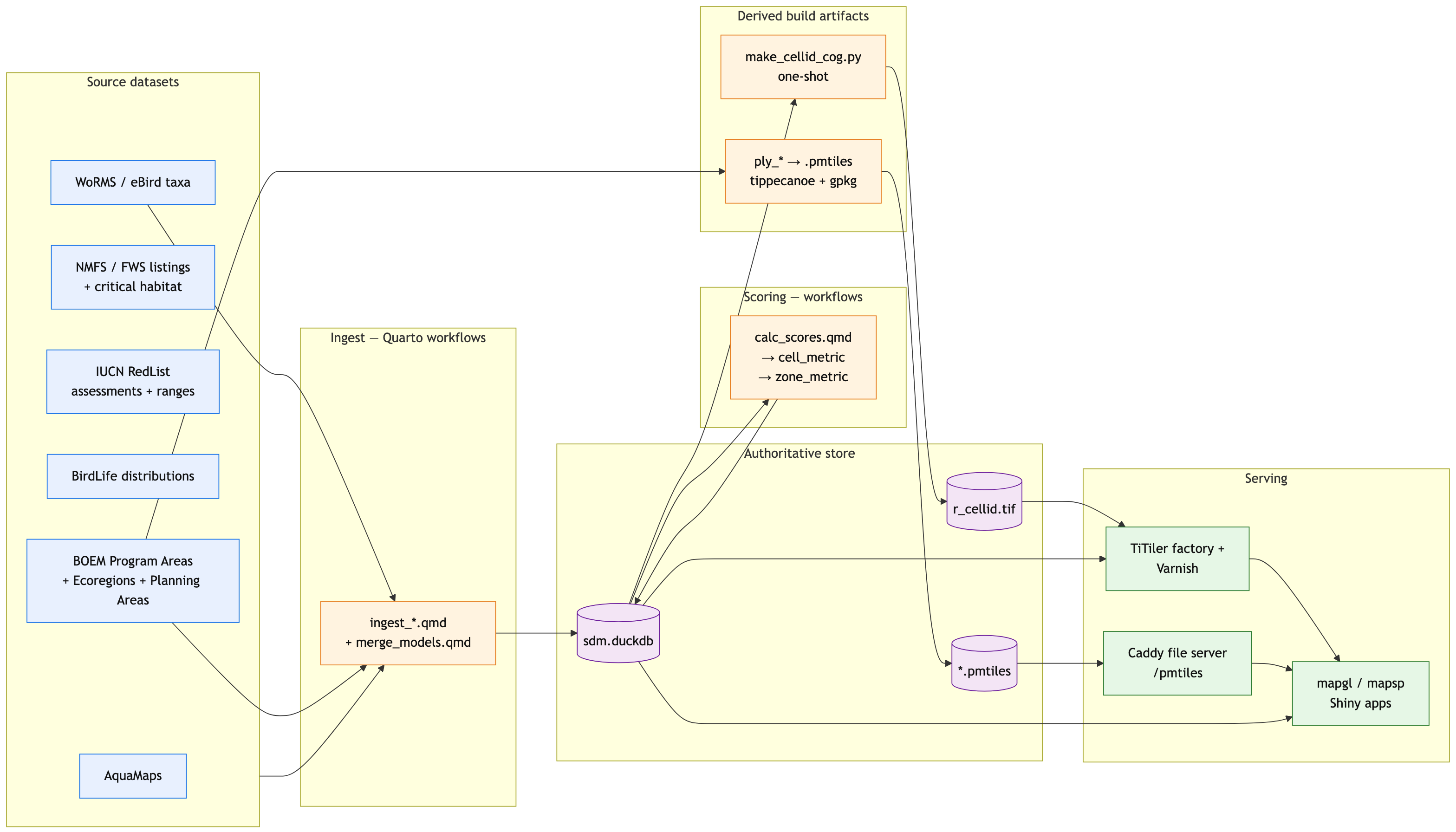
The serving paths above all sit downstream of one pipeline: ingest workflows write per-dataset distributions, the merge workflows combine them into one surface per taxon, the scoring workflows compute cell_metric and zone_metric, and the release workflow publishes the result as partitioned Parquet plus COGs, PMTiles and a STAC catalog. The whole thing is a targets graph generated from each notebook’s own metadata, so adding a dataset means adding a notebook (Figure 12.5). See Chapter 15.

Figure 12.5: Data pipeline: ingest workflows populate DuckDB; scoring workflows compute cell_metric and zone_metric back into DuckDB; a one-shot COG regen and offline PMTiles build produce the derived artifacts the serving tier reads.

12.1.3 Github Repositories

repo	description
.github	organization README
analytics	NA
api	application programming interface (API) using R Plumber package
apps	Shiny applications
docs	documentation for BOEM’s offshore environmental sensitivity index products
manuscripts	Manuscripts with review of sensitivities by industry and receptors (species, habitats, human uses)
MarineSensitivity.github.io	default website
msens	R library of functions for mapping marine sensitivities, sponsored by BOEM
objectives	repository for issues spanning multiple repositories and doing big picture roadmapping
server	server setup for R Shiny apps, RStudio IDE, Caddy web server, h3 TiTiler service and Varnish cache
stac-sdm	STAC extension for Species Distribution Models (SDMs)
workflows	scripts for testing data analytics and visualization as well as production workflows

12.1.4 Software Components

Chang, Winston, Joe Cheng, JJ Allaire, et al. 2024. Shiny: Web Application Framework for r. https://CRAN.R-project.org/package=shiny.

Lowndes, Julia S. Stewart, Benjamin D. Best, Courtney Scarborough, et al. 2017. “Our Path to Better Science in Less Time Using Open Data Science Tools.” Nature Ecology & Evolution 1 (6): 0160. https://doi.org/10.1038/s41559-017-0160.

Maitner, Brian, Paul Efren Santos Andrade, Luna Lei, et al. 2024. “Code Sharing in Ecology and Evolution Increases Citation Rates but Remains Uncommon.” Ecology and Evolution 14 (8): e70030. https://doi.org/10.1002/ece3.70030.

Wilkinson, Mark D., Michel Dumontier, IJsbrand Jan Aalbersberg, et al. 2016. “The FAIR Guiding Principles for Scientific Data Management and Stewardship.” Scientific Data 3 (1): 160018. https://doi.org/10.1038/sdata.2016.18.