| Metric | Description |
|---|---|
extrisk_bird |
Extinction risk for bird |
extrisk_bird_ecoregion_rescaled |
Extinction risk for bird, rescaled to [0,100] based on Ecoregional min/max values |
extrisk_coral |
Extinction risk for coral |
extrisk_coral_ecoregion_rescaled |
Extinction risk for coral, rescaled to [0,100] based on Ecoregional min/max values |
extrisk_fish |
Extinction risk for fish |
extrisk_fish_ecoregion_rescaled |
Extinction risk for fish, rescaled to [0,100] based on Ecoregional min/max values |
extrisk_invertebrate |
Extinction risk for invertebrate |
extrisk_invertebrate_ecoregion_rescaled |
Extinction risk for invertebrate, rescaled to [0,100] based on Ecoregional min/max values |
extrisk_mammal |
Extinction risk for mammal |
extrisk_mammal_ecoregion_rescaled |
Extinction risk for mammal, rescaled to [0,100] based on Ecoregional min/max values |
extrisk_other |
Extinction risk for other |
extrisk_other_ecoregion_rescaled |
Extinction risk for other, rescaled to [0,100] based on Ecoregional min/max values |
extrisk_turtle |
Extinction risk for turtle |
extrisk_turtle_ecoregion_rescaled |
Extinction risk for turtle, rescaled to [0,100] based on Ecoregional min/max values |
primprod |
Primary productivity: Oregon State Vertically Generalized Production Model (VGPM) from Visible Infrared Imaging Radiometer Suite (VIIRS) satellite data (mg C / m^2 / day) from daily averages available as monthly averaged to annual and averaged to overall for the most recently available full years of data 2014 to 2023 |
primprod_ecoregion_rescaled |
Primary productivity rescaled to [0,100] based on Ecoregional min/max values |
score_extriskspcat_primprod_ecoregionrescaled_equalweights |
Combined score of extinction risk per species category and primary productivity, equally weighted (and each previously rescaled [0,100] based on Ecoregional min/max values) |
10 Scoring
Scoring turns merged species distributions and extinction-risk weights into per-cell sensitivity metrics, which are then rescaled within ecoregions and aggregated to management zones.
TipInteractive walkthrough
The Scoring Walkthrough animates this pipeline — input rasters, merge, ecoregional rescaling and component averaging, step by step.
10.1 Cell-level scoring
For each cell, sensitivity is the extinction-risk-weighted sum of species presence within a species category:
\[ \text{score}_{c,g} = \sum_{s=1}^{S_g} \frac{\text{er\_score}_s \times v_{s,c}}{100} \tag{10.1}\]
where \(\text{score}_{c,g}\) is the score for cell \(c\) and category \(g\); \(\text{er\_score}_s\) is species \(s\)’s extinction-risk weight (1–100, Chapter 8); \(v_{s,c}\) is the merged model value for that species in that cell (0–100, Chapter 9); and \(S_g\) is the number of valid species in the category. Dividing by 100 returns the product to a 0–100 scale.
In plain terms: for every cell the MST adds up the contributions of the species found there. A cell holding many species that are both likely present and at high risk scores higher — which is how places where rare or threatened species concentrate are identified.
10.1.1 Two exceptions: species whose risk varies across the range
For sea turtles, extinction risk is already inside the merged values via the multiplicative merge (Chapter 9), so the formula collapses to a plain sum:
\[ \text{score}_{c,g} = \sum_{s=1}^{S_g} v_{merged,s,c} \tag{10.2}\]
er_score = 100 acts as a pass-through multiplier that cancels against the division. Cells inside an Endangered DPS therefore contribute more than cells inside a Threatened one, for the same species at the same suitability.
For the NMFS DPS-listed species (the humpback whale, Southern Resident killer whale, salmonid ESUs, …) the merged value is the suitability alone and the risk is a per-cell weight carried beside it, so the species-level er_score is replaced by the cell’s:
\[ \text{score}_{c,g} = \frac{1}{100} \sum_{s=1}^{S_g} er_{s,c} \times v_{s,c} \tag{10.3}\]
Numerically this is the turtle product taken one step later; the difference is that the merged model these species publish is their distribution, not their risk-weighted distribution. Each taxon’s rule is recorded as er_mode in the scoring taxon table (taxon — the scalar weight; premultiplied — sea turtles; cell — DPS-listed species).
10.2 Metrics
One extinction-risk metric exists per scored species category — invertebrate, fish, other, bird, coral, mammal, turtle — plus primary productivity, which carries no extinction-risk weighting.
10.3 Ecoregional rescaling
Raw cell scores vary naturally between ecoregions, through differences in species richness, oceanography and biogeography. Each metric is therefore rescaled to 0–100 within each BOEM Ecoregion:
\[ \text{score}'_{c} = \frac{\text{score}_{c} - \text{score}_{min}}{\text{score}_{max} - \text{score}_{min}} \times 100 \tag{10.4}\]
with the minimum and maximum taken over that metric’s cells within the ecoregion.
ImportantScores are relative within an ecoregion, never absolute
A score of 100 marks the most sensitive cell for that metric within that ecoregion — not globally. A 30 in Alaska and a 30 in the Pacific describe different ecological contexts.
Scores are therefore directly comparable among Program Areas within one ecoregion, and should not be compared across ecoregions.
Why rescale at all? Without it, naturally species-rich areas would almost always score highest simply for holding more species. More species may well indicate greater ecological importance — but it can equally be argued that the fewer species an ecosystem has, the more each one matters to its function and resilience. Rescaling within ecoregions keeps scores from being dominated by richness. Comparing across ecoregions would require settling that argument with a mathematical relationship between the two views, which remains a live academic debate.
10.4 Spatial units
| Unit | Field | Count | Vintage |
|---|---|---|---|
| BOEM Ecoregion | ecoregion_key |
12 | ecoregion_2025-06 |
| BOEM Planning Area | planarea_key |
36 | planarea_2025-06 |
| BOEM Program Area | programarea_key |
20 | programarea_2026-01 |
| Subregion | subregion_key |
5 | subregion_2025-06 |
Geometry is versioned by its own vintage rather than by release, so several releases legitimately share one boundary set — one Program Area geometry covers v2 through v8, and one ecoregion geometry covers every release. Each release’s manifest names the vintage it used, which is what lets this book draw the correct outlines for the version it documents instead of the newest ones.
10.4.1 Geographic scope
The analysis covers 20 BOEM Program Areas from the 11th National Draft Proposed Program (2025), spanning Alaska, the Pacific and the Gulf of America. The Atlantic OCS is not part of this program cycle, so ecoregions containing no Program Area are outside the scored footprint.
The Gulf of America Program Areas (GAA and GAB) each span two ecoregions — Western and Central Gulf of America, and Eastern Gulf of America. Because rescaling happens before aggregation, cells are rescaled against their own ecoregion’s range, and the Program Area score is then the area-weighted mean across all its cells regardless of ecoregion. Local ecological context is preserved even where a Program Area crosses a boundary.
10.5 Primary productivity
Net primary productivity from the VGPM satellite model enters as its own metric (primprod), without extinction-risk weighting. The raw values (metric tons C km-2 yr-1) are rescaled within each ecoregion on the same 0–100 basis as everything else.
10.6 Zone aggregation
Rescaled cell scores are aggregated to each spatial unit by area-weighted mean:
\[ \text{score}_{zone} = \frac{\sum_{c \in zone} \text{score}'_c \times A_c}{\sum_{c \in zone} A_c} \tag{10.5}\]
where \(A_c\) is the area of cell \(c\) — which is latitude-dependent on a 0.05° grid, so the weighting is not cosmetic.
10.7 Visualization
10.7.1 Flower plot
The flower plot summarizes a zone’s sensitivity profile by category, after the Ocean Health Index (Halpern et al. 2012):
- petal length — the rescaled score (0–100) for that category; longer means more sensitive
- petal width — that category’s weight in the composite; wider means more influence
- centre — the weighted mean across categories
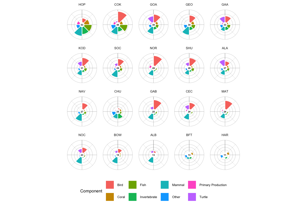
It lets a reader see at a glance which ecological elements drive sensitivity in an area. The scores app implements an interactive version.
10.7.2 Treemap
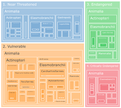
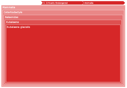
The treemap shows how individual species contribute to a score, nested first by extinction-risk category and then by taxonomy, with zoom down to single species.
10.7.3 Score rasters
Cell-level scores are published as Cloud-Optimized GeoTIFFs, one per metric x subregion, with the manifest carrying each raster’s URL and its build-time rescale range. The map reads those directly.
This replaced a tile factory that ran SQL against the database on every tile request. The rasters were verified byte-identical to the factory’s output before the switch. They are stored without overviews deliberately: the renderer decimates from full resolution per request, so a pre-built pyramid would disagree with it at low zoom.
10.7.4 Interactive maps
Two Shiny applications present the results, each rendering any published release from the URL path rather than being frozen to one:
- Scores — composite and per-category sensitivity by zone, with flower plots and treemaps (see Appendix C)
- Species — individual and merged distribution models with regulatory status (see Appendix D)
Substitute the version in the path (e.g. /v3/scores/) to view that release; an older ?ver=v3 deep link still resolves, 301’d to the equivalent path. See Chapter 19.
10.8 Implementation
Scoring runs in the score_zones, score_cell_metrics and score_zone_metrics workflows (Chapter 16). Whole-pipeline equivalence between releases is checked by msens::pra_score_delta, which compares Program-Area scores on the species the two releases share.