Appendix A — Atlas (beta) — the static, in-browser scores, species and places app

B Atlas

B.1 Overview

The Atlas (https://marinesensitivity.org/atlas/?ver=v7) is a third, newer way to explore the MST, currently labelled beta: one static web app, built with Svelte and MapLibre, that runs entirely in the browser. Where the Scores and Species Shiny apps are server-rendered R processes, the Atlas has no application server of its own: scores, flowers, tables and reports are computed in your browser, by a DuckDB instance compiled to WebAssembly (DuckDB-WASM) querying the release’s published Parquet directly over HTTPS. It still depends on a few other services for what a browser cannot compute itself — score and species map tiles come from the project’s titiler, zone outlines from PMTiles on S3, and the basemap from CARTO — but there is no Atlas-specific backend.

On the public host the release is a query parameter (?ver=v7), resolved client-side against the published versions.json and defaulting to the promoted release when absent. A restricted pre-release is served the same way the preview Scores and Species apps are, at https://preview.marinesensitivity.org/{ver}/atlas/ (the version as the URL path, since Cloudflare Access scopes its reviewer policies by path, never by query).

Figure B.1 shows the default Scores view: the 0.05° cell grid colored by a composite sensitivity score across U.S. waters, dark theme (the app’s default), with the tool rail on the left, the Layers panel open by default, and the basemap’s attribution in the lower-left corner.

Figure B.1: The Atlas, Scores lens, default view (desktop, dark theme).

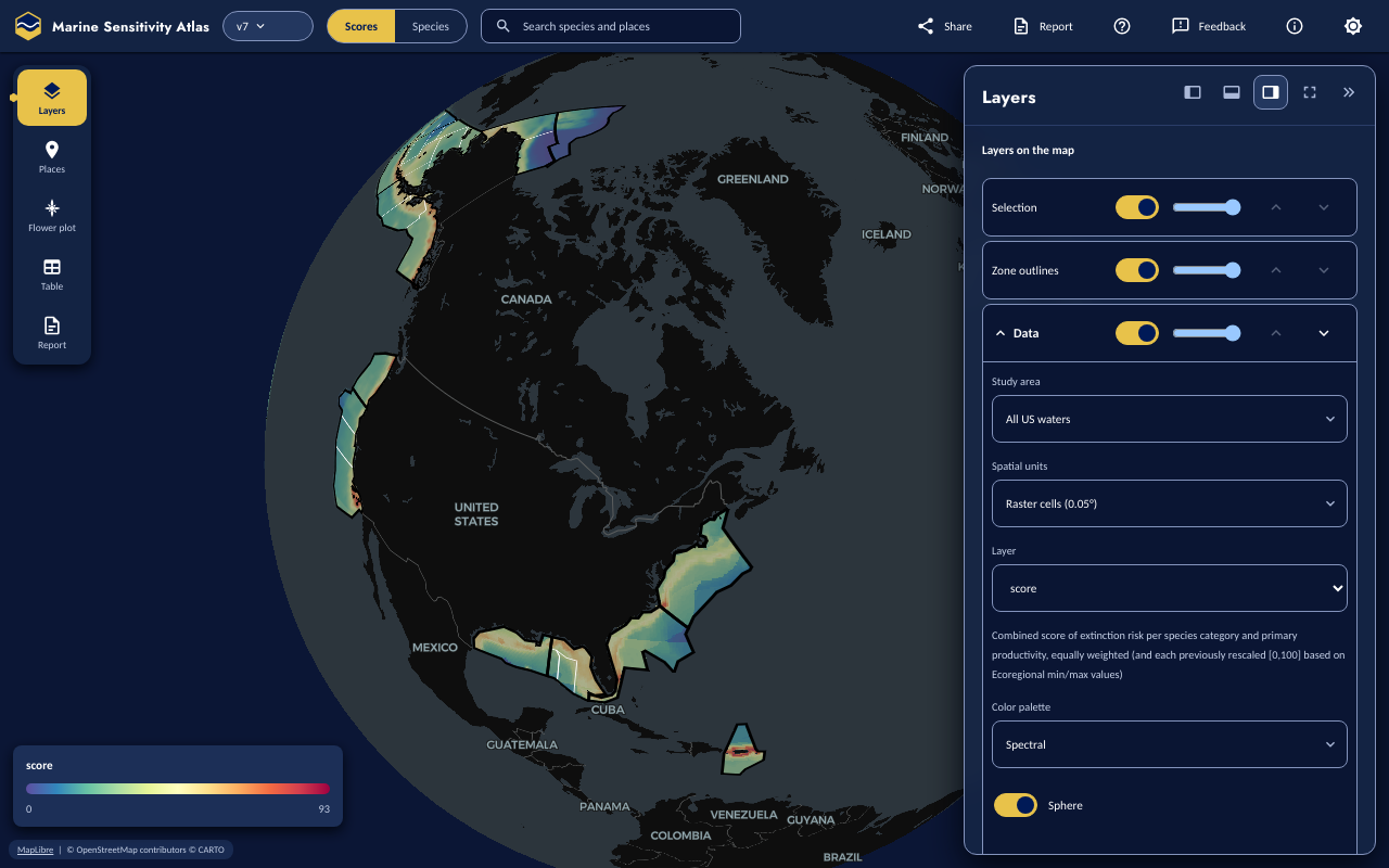
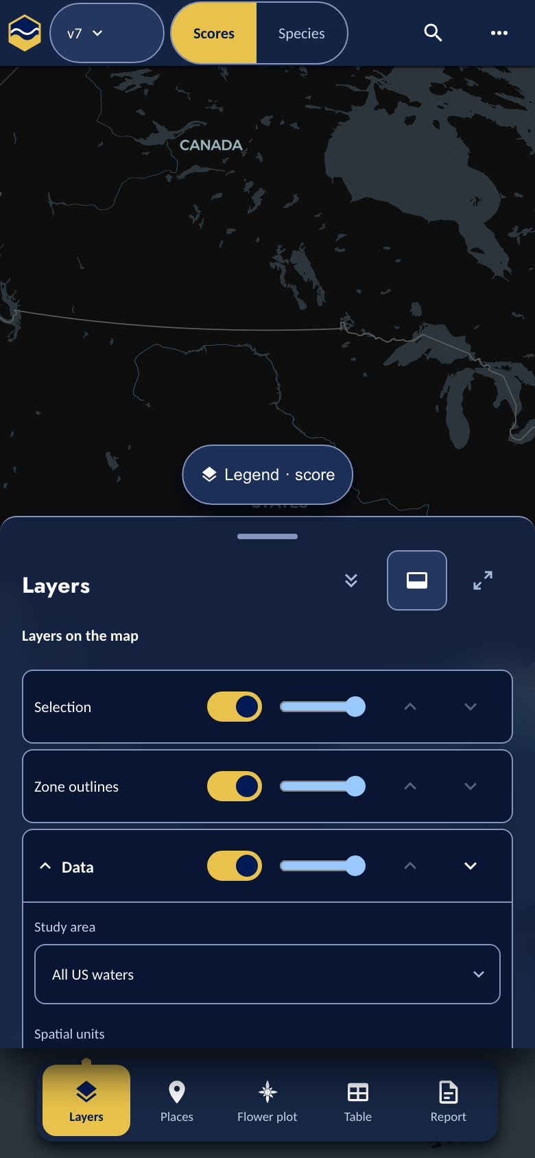
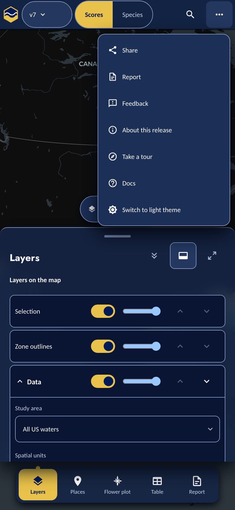
Desktop vs. phone layout. On a wide viewport the five rail tools open a single dockable panel that floats over the map; on a phone the identical five tools sit in a labelled bottom tab bar, and the panel becomes a bottom sheet with three heights (peek, half, full). Figure B.2 shows the phone layout, and Figure B.3 its top bar’s More (⋯) menu.

Figure B.2: Phone: default view.

Figure B.3: Phone: the top bar’s More (⋯) menu.

B.2 Quick start

Desktop:

1. Open Places, and either choose a Program Area from its list or draw a Rectangle (click, move, click, then Done).
2. Select the place in the list — Program Area or drawn — to see its results: a coverage note (or, for a Program Area, its published cell count, area and composite), a flower and component table, and (on request) its species table.
3. Rename it inline if you like.
4. Places › Share › Copy link — the fastest way to hand someone the same place.
5. Places › Report for a printable, downloadable document (Print, HTML, ZIP or Word).

Phone: the tool rail is the bottom tab bar; use the Program Area chooser or Enter coordinates rather than drawing, and the file picker rather than dropping a file on the map (that gesture needs a desktop pointer).

B.3 Getting around

The top bar, left to right on desktop: the MST mark and title; a release chip that opens the version picker; a Scores | Species lens switch; a search field (Program Areas and coordinates in the Scores lens, Section B.4; species in the Species lens); then, right-aligned, Share, Report, a (?) Help menu (Take a tour, keyboard shortcuts, a Docs link), a Feedback button, an (i) About button, and a sun/moon theme toggle. On a phone (below 900 px) the title collapses to the mark, and Share, Report, Help, Feedback, About and the theme toggle fold into one More (⋯) button beside a search button; below 381 px the mark hides too. The keyboard-shortcut list is desktop-only.

The tool rail is five controls, always in the same order, on every viewport: Layers · Places · Flower plot · Table · Report. In the Species lens the Flower control fades in place — it has no meaning for a single species — but stays visible with a tooltip explaining why.

The panel that a rail tool opens is one dockable surface: dock left, right or bottom; resize by dragging its map-facing edge or with arrow keys; maximize to the whole stage; or collapse to a small labelled pill (clicking any rail tool re-opens it). Its dock/size/collapsed state is chrome, remembered per viewport, never written into the shareable URL. On a phone the same panel is the bottom sheet, with peek/half/full detents. On a desktop the map’s legend floats in a corner clear of the panel, on whichever side it is docked, and hides while the panel is maximized; on a phone it is a compact Legend chip above the sheet that opens the full legend, moving into the sheet’s own header at full height.

B.4 Scores lens

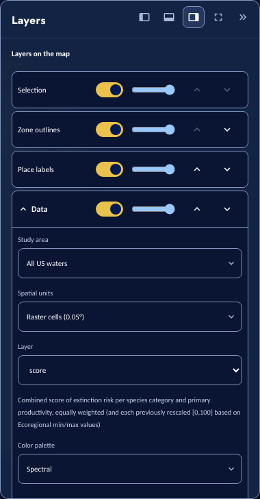
The Scores lens shows the composite, extinction-risk-weighted score for every 0.05° cell (or, aggregated, every Program Area) of U.S. waters. Opening Layers (Figure B.4) expands the Data row into this lens’s own controls — study area, spatial unit, the score layer, color palette, a Sphere switch (globe vs. flat projection), and a Cells outside Program Areas switch where the release publishes that overlay — above the rest of the layer stack, listed top to bottom: Selection (pinned at the top), Zone outlines, Data, Place labels, Roads & buildings, Boundaries, Bathymetry (present but disabled until a relief layer is published) and Land & water at the bottom. Every row’s visibility and opacity can be changed, and most can be reordered — Data can never move above Zone outlines, so an opaque score raster can never hide the boundaries it is measured against — and Reset layers restores the default stack.

Figure B.4: The Layers panel docked, with Place labels moved above Data (one “move up” click) to show the reorder feature, and Data expanded to its study area, spatial units, layer and palette controls.

Clicking a cell or a Program Area selects it: the URL gains a sel=cell:<id> or sel=zone:<unit>:<key> token, which the Flower plot and Table tools then describe (Section B.8). A click on land or outside the scored area shows “No scored cell here” with its coordinates and leaves the selection unchanged.

The top-bar search field also works here: it matches Program Areas (and any subregion/ecoregion archive the release happens to publish) by key (“ALA”) or by name (“Aleutian”), and coordinates typed as “lon, lat” (e.g. “-140, 57” — “lat, lon” is read correctly too, either by an explicit lat/lon label or because the default order would be out of range). Matching is entirely offline, against only what the release itself already publishes — no Nominatim, no third-party geocoder, no network call. Choosing a Program Area result selects it exactly as clicking it on the map would, and flies the camera there; choosing a coordinate result flies to the point and selects that cell. Results are a keyboard-navigable list (arrow keys, Enter to select, Esc to close), on both the desktop top-bar field and the phone’s search modal.

B.5 Species lens

Switching to Species turns the top-bar search into a species picker (common or scientific name, with an “Only species in US waters” checkbox), and replaces the Data row’s contents inside Layers with the species card: the merged model as a filled pill marked ✓ with a gold edge, plus one pill per contributing input dataset marked ▶ with a grey edge. An input’s raster is found the same way the Species Shiny app finds it — through the release’s model-asset registry, looked up by model key — and an input whose registry row is missing renders as a struck-through, non-interactive pill, never simply omitted. Where the selected input publishes both, one representation toggle appears (“Original” vs. “Interpolated,” or “Delivered” vs. “As ingested” for a dataset already on the scoring grid). Selecting a species flies the map to that model’s extent; clicking it then returns that cell’s modelled value, or “No scored cell here” outside the model’s range. The legend floats in a corner of the map (a legend chip on a phone), titled with the species’ scientific name and its 1–100 range.

Figure B.5: The Species lens’ card for the leatherback turtle (Dermochelys coriacea): the merged model with every one of its six inputs struck through — as of this writing, a stale v7 app bundle rather than a genuinely missing registry row for all six (see Known Limitations).

B.6 Places

Places is the tool the two Shiny apps do not have: any area you outline gets the same scores and species results the built-in Program Areas get. The empty state reads exactly: “No places yet. Choose a Program Area above, turn on pick mode and click one on the map, draw a shape, enter coordinates, or drop a file on the map.”

• Pick a Program Area. Turning on pick mode and clicking only highlights it — Ctrl/Cmd-click, Shift-click or long-press to highlight several — and “Add to places (n)” is the button that actually adds it; several picks become one place. Or use the panel’s own Program Area chooser, which needs no pointer and works on a phone. Program Areas are shown as “Full Name (KEY)” — e.g. “St. George Basin (GEO)” — from an app-side name table generated off the canonical Program-Area geometry (no published release, v6 through v9, actually publishes a full name on its own Program Area rows; a release that does publish one is preferred when present), in the Places panel, the Scores-lens search and the Zones table and report; from 0.10.59, everywhere — today the Scores-lens map tooltip, Flower title and Table header for a clicked Program Area still show the bare key.
• Draw a Polygon, Rectangle or Circle: click, move, click for each vertex or corner (not a drag), then press Done — a polygon also closes when you click its first vertex again, or press Enter. A circle is stored as a 64-sided polygon. Dragging a finished shape’s corner edits that place in place (same row, same name, re-analysed) rather than adding a new one.
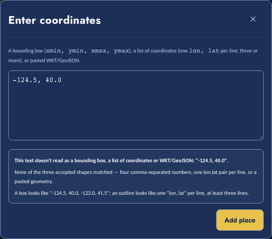
• Enter coordinates — the keyboard/screen-reader alternative to drawing, in a modal dialog: a bounding box (xmin, ymin, xmax, ymax), a list of lon, lat vertices one per line, or pasted WKT/GeoJSON. A refusal is shown verbatim — what went wrong, why, and how to fix it.
• Upload a file, through the picker or by dropping it anywhere on the map: “GeoJSON, zipped shapefile, KML, GPX, FlatGeobuf, WKT or GeoPackage, up to 10 MB.” GeoPackage is now read (polygons only, same as every other format), through the same resident DuckDB-WASM engine the scores boot, via its spatial extension — fetched live, with consent, from extensions.duckdb.org (the one deliberately non-mirrored third-party download, 22.4 MB); each .gpkg upload asks first, not just the first one in a session. A GeoPackage with no vector layer (raster tiles, or a plain attribute table) is refused when ST_Read fails to read it (see Known limitations), not by a dedicated check. Other rules that cause a refusal: polygons only (points and lines are refused, never buffered); a shapefile needs its .prj (projected coordinates are refused); at most 50,000 vertices; a zipped shapefile at most 50 MB uncompressed and 200 entries; and the shape must touch the U.S. study area. A feature’s own name (KML’s <name>, or a name/title/label property on GeoJSON/shapefile/etc., case-insensitive) — auto-detected from the file’s first feature and applied to every feature — names each place; a file with no such property falls back to the file name, numbered. A file with several features becomes one place per feature (up to 20), each named this way, or one merged place, named after the file, your choice.

Figure B.6: The Places panel with two places, both analysed: a Program Area (“Aleutian Arc (ALA),” 875,225 km², 28.3 composite) and a selected, entered-coordinates place (“bounding box,” 98,973 km², 100% coverage, 27.1 composite) whose coverage note reads “100.0% of this place is inside the US study area (3,600 of 3,600 cells)”; the drop zone above the list names the accepted formats, GeoPackage included. Captured on 0.10.62.

Figure B.7: The “Enter coordinates” dialog, showing a refusal for input that matches none of the three accepted shapes.

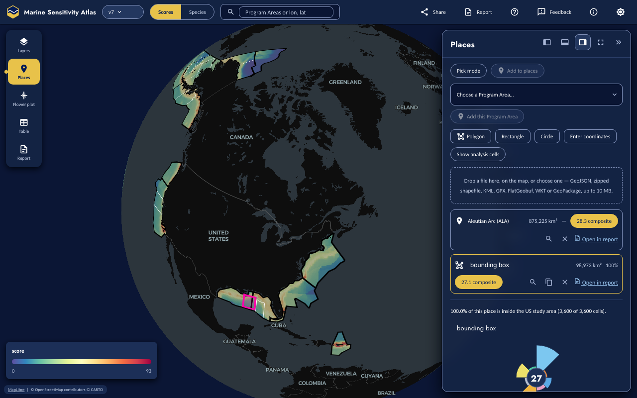
Each row shows its area and, as soon as it is analysed, its data coverage percentage and composite score directly in the row — for a drawn, typed or uploaded place the same analysis runs for every such place in the list, not only the one currently selected; a Program Area row shows its own published composite the same way (e.g. “Aleutian Arc (ALA) … 28.3 composite”). Row actions: an inline rename (≤ 60 characters, drawn/uploaded places only), zoom to, duplicate (drawn/uploaded only), delete, and Open in report. Selecting any place — drawn, typed, uploaded, or a Program Area — expands the same results panel below the list, though the note at its top differs by kind: a drawn, typed or uploaded place shows a coverage note (“N% of this place is inside the US study area (a of b cells)”, or “This place is outside US waters here: no scores can be computed”); a Program Area shows its own note instead (“N cells, A km²; published composite C.”). Both then show a flower plot and a component table, and a species table on request — a drawn/typed/uploaded place behind a “Loading species needs N tiles, about X MB. Continue?” prompt (species come from map tiles), a Program Area behind a plain Load species button with no such prompt (its species table is a precomputed release table, not tiles). A single selected Program Area reads all of this straight off the release (the same path the Scores lens’s Table › Zones tool uses, Section B.8); a multi-Program-Area selection (several picks added as one place) still sums area and means the composite for the list row, but its flower/component/species panel asks you to select a single Program Area instead of guessing which one’s to draw. Show analysis cells paints the analysed 0.05° cells (up to 20,000 of them) for a drawn, typed or uploaded place; for a Program Area it reads plainly “Show analysis cells: not available for Program Areas yet” — the app bundle the Atlas reads does not yet carry per-zone cells, even though the release’s own tables do (see Known limitations) — rather than showing a disabled control with a misleading reason. The list caps at 20 places (“n / 20 places”); Recent (this browser only) offers to add a removed place back. The footer holds Share, Download places (GeoJSON) and Report, each disabled with zero places.

Two different Share buttons. The top-bar Share simply copies the current address bar to the clipboard — no dialog, no summary, no length check. Places › Share opens the real dialog described next, and is the one to use whenever places are involved.

B.7 How places are stored in the link

A place never lives on a server: it is encoded directly into the URL fragment (#pl=, never the query string, so it is never sent to a server or a referrer), so opening a shared link reproduces the sender’s exact area. Every analysis runs on the decoded geometry, never the geometry as drawn, so the numbers can never diverge between sender and recipient. Places are joined with ~:

#pl=z.pa.GAA~g1.Gulf%20box.EAMBAQSf_grYrQPQDwAA0A_PDwA

(the decoded form; the address bar itself percent-encodes ~ and other reserved characters)

• z.<set>.<key>[,<key>...] — a reference to a built-in zone (pa Program Area, pl Planning Area, er ecoregion, sr subregion); its geometry comes from the release’s own PMTiles.
• g1.<name>.<base64url bytes> — a drawn, typed or uploaded polygon, carried inline as a compact binary encoding (see “For developers” below).
• u.<name>.<8-hex-digit digest> — the fallback for a place too large to carry (see below): only a name and a digest travel.

NoteFor developers: the g1 byte layout

Each ring is quantized to a fixed precision (3 decimal digits, ~110 m — 4 digits when the place’s bounding box is under 0.5° in both directions), delta-encoded vertex-to-vertex as zigzag varints running across rings and polygons, and base64url-encoded with no general-purpose compression (delta varints are already dense). Longitudes are stored unwrapped, so a place crossing the antimeridian round-trips without a special case. msens::place_decode() is the R decoder; the shared test fixture (tests/fixtures/place_codec.json) matches it byte for byte.

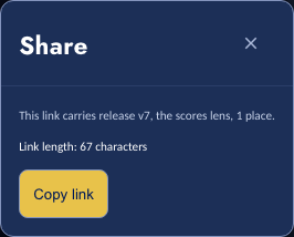
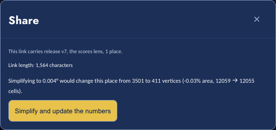
The link’s length is checked only when you open Places › Share. Adding a place, or copying the top-bar Share link, carries the unsimplified geometry (already quantized to 3–4 decimals) regardless of length. In that dialog: up to 2,000 characters silently; between 2,000 and 8,000 a note reads “This link is over 2,000 characters — some chat apps and older browsers truncate very long links,” with Copy anyway; only above 8,000 does the Douglas-Peucker ladder run — 0.001° doubling to 0.016°, a rung accepted only while the area changes by no more than 1% and every ring stays simple — aiming to bring the link back under 2,000 characters; it stops at the first rung that does, or, if none does, uses the coarsest accepted rung provided that still fits under 8,000. This is never silent: the dialog shows the before/after (vertices, area change, cells, Figure B.9), and you click “Simplify and update the numbers” to accept it — which is also what rewrites #pl=, so the copied link and the displayed numbers can never disagree. If even the coarsest rung is still too long, Copy link anyway copies every drawn, typed or uploaded place (zone places are unaffected) as a u. token instead — your own address bar and session keep the real shapes; the recipient of that copied link sees a named row with no results and a “not analysed yet” chip, never a prompt. The dialog’s own advice at that point is to download the place as GeoJSON and send that alongside the link. A single small rectangle almost always fits in the silent budget; that is not guaranteed for several places together, or a long base URL.

Figure B.8: The Share dialog: what the link carries and its exact length.

Figure B.9: The Share dialog’s simplification ladder for an oversized place: before/after vertex count, area change and cell count, with a “Simplify and update the numbers” button.

The rest of the view travels the same URL-is-the-state way, in the query string: ver, lens, lyr/sp, unit, area, map (camera), pal, sel, layers (the stack deltas from Section B.4), theme and tour — each written only when it differs from its default.

B.8 Flower plot and Table

Flower plot and Table are Scores-lens tools for a clicked cell or Program Area; in the Species lens, Table is a placeholder, and a drawn Place’s flower and species table live in the Places results panel instead (Section B.6), not here.

The flower draws one equal-width annular petal per score component, scaled to its rescaled score; the hub shows the plain mean of the components present (not a weighted mean). Since 0.10.41 the values also list in a real table (swatch, component, score, and a Mean row) below the plot.

Figure B.10: The Flower plot for a clicked cell in the Gulf of America: one petal per score component, and the values table with a Mean row below it.

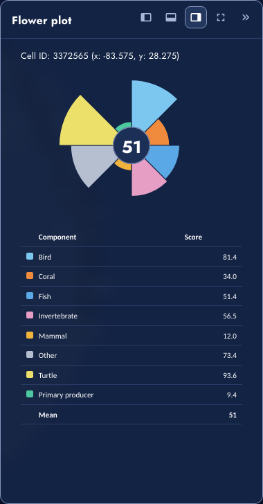
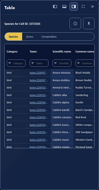
Table opens three tabs: a sortable species table (Category, Taxon, Scientific name, Common name, ER code, ER score, Model, MMPA, MBTA, Area (km²), Avg. suitability, % of category — ESA and IUCN status are folded into ER code), a zones table (every Program Area ranked by the current layer, with “report on selected” once some are ticked), and a composition treemap (one box per species category, sized by suitability × extinction risk × area). Only the species table has the phone’s compact default columns and a Columns control; both tables get sticky headers/first column and horizontal scrolling that never spills the panel. Only the species table’s Download CSV exports it; the zones table and the composition treemap have no export yet. A drawn place’s Components and Species tables in the Places results panel each have their own working Export CSV.

Figure B.11: The Table tool’s species tab.

B.9 Report

Report reports every place currently in the link (#pl=); with no places, it reports the single selected Program Area; with neither, it shows a chooser. A row’s own Open in report reports just that row’s place. The document renders progressively as its data arrives:

• a header band — mark, release chip, generation time, permalink and QR code (a restricted release also gets a PREVIEW banner and print watermark);
• an introduction;
• a collapsible Parameters section (kind, keys or vertices, area, cell count, study-area share, token);
• a map — interactive on screen; a static snapshot only in print and the HTML export;
• one flower plot per place, under “Plot of Scores”;
• a Table of Scores — component and overall scores, with a footnote when a component covers under 99% of the area, or is missing entirely because the release’s own 5% coverage floor dropped it;
• a Summary of Species per place (a category × count cross-tab, plus the top 20 by score);
• Sources and Method, with the release’s own citations — each query behind these numbers is a parity-tested twin (npm run parity, max|Δ| < 1e-9) of an msens R function; “Reproduce in R” prints the exact calls to msens::place_decode(), cells_in_polygon_grid() and scores_for_cells() that reproduce it, needing msens ≥ 0.44.0 and a local copy of the release’s sdm.duckdb;
• a Provenance section (release, status/access, app build SHA, DuckDB-WASM version, tables read, SQL run).

Figure B.12: The report document’s header band and introduction: the MMA seal, a permalink and QR code, Parameters, and the start of the interactive map.

Figure B.13: The report’s Table of Scores and the start of the Summary of Species, for the same Program Area.

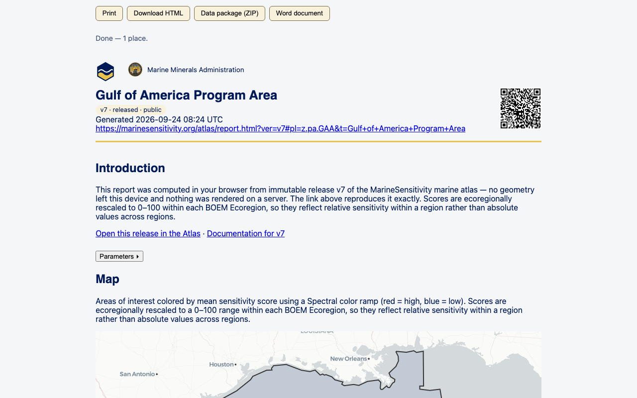
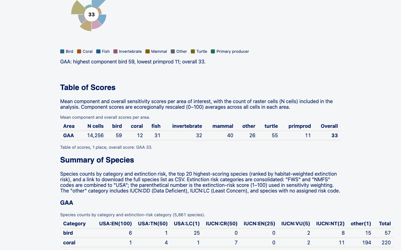
Four exports, all built client-side: Print (the browser’s dialog; roughly five Letter pages); Download HTML (one self-contained file — the flowers stay inline SVG, only the map is an embedded PNG); a data package (ZIP) — README.md, CITATION.md, provenance.json, places.geojson (drawn/uploaded places only, not zone places), a scores_*.csv/species_*.csv pair per place, and query/*.sql; and a Word document (.docx) — the same tables as coded Word styles, plus the map and a rasterized flower per place.

B.10 Accessibility and performance notes

The Atlas ships a written WCAG 2.1 conformance note and a performance budget report in its own repository. As of the note’s own 0.10.24 (2026-09-23) evaluation the claim is “partially supports,” not full support, and it states plainly that no screen reader was actually driven in producing it — automated and manual keyboard testing stand in for that. Two skip links sit at the very top of the page: “Skip to the tools” and “Skip to the details panel.” The critical-path JavaScript was measured (0.10.20, 2026-09-23) at ~417 KB gzip against a 450 KB budget, plus ~140 KB for the MapLibre worker against 150 KB; a separate gate asserted the species lens paints its first data pixel within 2.5 s on a laptop and 4 s on CI. Both budgets may have moved since; see the linked reports for current numbers.

B.11 When a service is down

Since 0.10.59, the Atlas checks two external services it does not control: titiler-v8 (every score and species map tile) and the S3 data origin each release’s own files are fetched from. Both are checked at boot and on a manual Retry; a map tile that actually fails to load for a real reason — a 5xx, a network error, or a timeout, never a normal “this release has no data here” 403/404 — re-checks only the tile server. It never polls in the background while everything is fine.

When either is down, a dismissible top banner names the failing host, the reason (timeout or HTTP status), and what still works — places, tables and reports already built from data already loaded, just no new tiles or new fetches from the down host; when it is specifically the tile server that is down, the legend also switches to a compact “tiles unavailable” state instead of a bare colour ramp. Built 2026-09-24 after titiler-v8 and the API were unreachable for an hour and the live app kept rendering a perfectly normal-looking map with no raster and no word to anyone.

What it cannot detect: a partial outage (some tiles or objects failing, others not — only a further real request surfaces it), a degraded-but-200 response (a tile that loads but paints wrong data), or a preview session’s own restricted data prefix (the probe always checks the public bucket origin, not a signed-in override). No release the Atlas reads from calls a separate API today, so there is nothing of that kind to probe; DuckDB-WASM’s own Parquet fetches, PMTiles zone archives and the basemap are likewise outside this check’s scope — a partial CDN problem affecting only one of those would not trip the banner.

B.12 Feedback and versions

Feedback opens a dialog: a kind (bug / idea / question / data), a title, a description, an optional email, an annotatable screenshot, and a privacy checkbox (off by default) for including the current view’s link. Send is live: it posts to a Google Apps Script endpoint that writes a Sheet row, mails the team, and — for a public release — also files a public GitHub issue in MarineSensitivity/atlas with the screenshot attached (your email, if given, is never included in it); a restricted release never gets a public issue either way. An email, if given, is kept only in the team’s Sheet row and mail (plus a copy to you), never in the issue (see docs/feedback.md in the atlas repo for the dialog’s exact privacy wording). The original zero-backend fallback stays alongside Send, not replaced by it: “Open as GitHub issue” opens its own prefilled public issue, labelled by kind, with the screenshot copied to your clipboard to paste in — offered on every public release whether or not Send is configured, and the only option on a build with no endpoint set. Tell an analyst plainly: on a public release, both routes end in a public GitHub issue. A restricted release never offers the GitHub route; on a build with no endpoint configured it says plainly that “feedback cannot be sent from here right now.”

GA4 receives interaction events as well as page views, and the app also logs those same events to the batched usage-log Sheet the Shiny scores/species apps already write (app = "atlas" distinguishes its rows) — never the URL fragment, which the app’s own analytics code is source-scanned to never read.

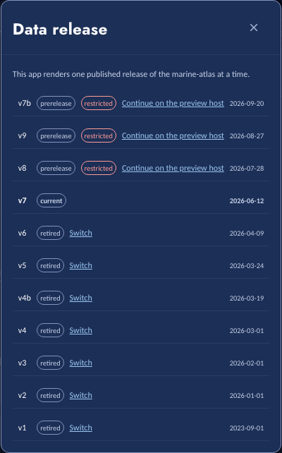
Versions follow the same public/restricted split as the rest of the MST (see Chapter 2): a public release opens directly on the public host; a restricted pre-release’s Atlas is reached only through the signed-in preview host, at its own /{ver}/atlas/ path. Requesting a release the current host cannot show opens the version picker automatically: a restricted one offers “Continue on the preview host” (from 0.10.59, that link goes straight to the Atlas there), an unrecognized one reads “is not a version this host recognizes,” and either way the promoted release loads underneath while the picker explains why. In the picker, every public release other than the current one offers Switch.

Figure B.14: The release picker.

B.13 Known limitations (as of 0.10.59)

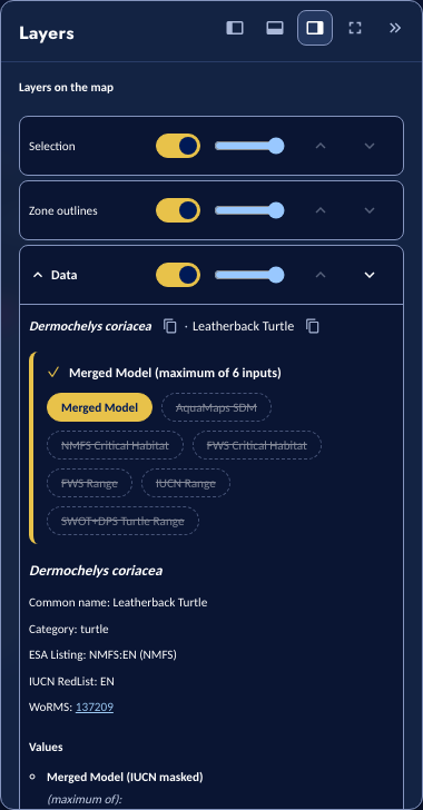
• For every release before v8 (v2–v7b), every input pill in the Species card still shows struck through, the leatherback’s six included (Figure B.5) — as of this writing, the app bundles that would resolve the model-asset registry lookup (see Species lens above) for 10,247 of v7’s 12,120 inputs have not yet been republished; once they land, only 1,873 of its 2,619 rng_iucn range inputs, which have no model-asset registry row (struck through in the Species Shiny app too), will still show this way.
• GeoPackage is refused (see the Places section above) whenever ST_Read fails to parse it, including a file with no vector layer — its declared-CRS and no-feature-table checks cannot actually run against an uploaded file, because DuckDB-WASM’s sqlite_scan() cannot open a file registered only through registerFileBuffer, the way an uploaded GeoPackage is, so both checks silently fall through and ST_Read, or the normal out-of-range magnitude check, is left to catch a projected or empty file instead (still refused, just by a different, honest rule).
• A multi-Program-Area selection (several picks added as one place) sums area and means the composite for its list row, but its flower, component table and species table are not aggregated — the results panel asks you to select a single Program Area for those.
• Show analysis cells is not available for a Program Area place: the app bundle the Atlas reads carries each zone’s count, area and scores but not its cells.
• The Atlas’s report is a print-first document built and exported entirely client-side (HTML/ZIP/DOCX from the same source), not the Shiny apps’ own report.

B.14 Generating Screenshots

The atlas repository’s own scripts/eyes-shots.mjs captures the standard states most of this chapter’s figures come from (18 numbered shots per viewport, about 11 states, phone 390×844 at 2x pixel density and desktop 1280×800, dark theme), run against a live or locally built app:

ATLAS_URL=https://marinesensitivity.org/atlas OUT=.tmp/eyes node scripts/eyes-shots.mjs

A few figures here (the Share dialog and its simplification ladder, the Coordinate dialog’s refusal state, the version picker, and one Report scroll position) are not among that script’s own states; they were captured by hand from the same live build, driving the app to the specific state each caption describes.

B.15 Source Code

atlas on its own main branch — one static build for every release, the same “one checkout, not one per version” convention the Scores and Species apps follow.