Abstract
The Bureau of Ocean Energy Management (BOEM) has developed the Marine Sensitivity Toolkit (MST), a cloud-native system for assessing the relative environmental sensitivity of marine ecosystems to offshore energy development across U.S. waters. Created specifically for BOEM’s National Oil and Gas Program, the MST integrates over 17,000 spatially explicit species distribution models, comprehensive extinction risk data, and satellite-based primary productivity to deliver a transparent, reproducible, and scalable assessment framework on a fine-scale 0.05° grid (~5 km cells). Sensitivity scoring combines species presence, extinction risk, and productivity, all rescaled within ecologically meaningful BOEM Ecoregions, supporting cell-by-cell analysis that captures nuanced ecological patterns often missed by coarser assessments. The MST is designed for transparency and rapid updates, ensuring that BOEM’s decisions are grounded in the best available science as mandated by Executive Order 14303: Restoring Gold Standard Science.
Background
The Bureau of Ocean Energy Management (BOEM) is legally mandated by Section 18(a)(2)(G) of the Outer Continental Shelf Lands Act (OCSLA) to consider “the relative environmental sensitivity and marine productivity of different areas of the OCS” when making decisions regarding oil and gas leasing and marine mineral development on the Outer Continental Shelf. This analysis is essential for guiding the timing and location of oil and gas lease sales and for implementing mitigation measures to minimize impacts on the marine environment.
In direct response to Executive Order 14303: Restoring Gold Standard Science (Federal Register, May 29, 2025), BOEM has modernized its approach by developing and implementing the Marine Sensitivity Toolkit (MST). This innovative, cloud-native toolkit fundamentally revamps BOEM’s previous Relative Environmental Sensitivity Analysis (RESA) (Morandi et al. 2018), delivering a transparent, reproducible, and scalable system that fully aligns with the Executive Order’s requirements for scientific integrity, transparency, and the use of best-available science.
The MST marks a significant advancement over prior RESA methodologies. Earlier approaches (Niedoroda et al. 2014) often relied on aggregated data from a limited set of broad species groups and surrogate species, lacking spatially explicit information for individual organisms. As a result, previous assessments were typically coarse and area-wide, frequently missing critical ecological variation and fine-scale patterns across the OCS. In contrast, the MST utilizes a high-resolution 0.05° grid (averaging 5 km in the lower 48 states and 3.6 km in Alaska), enabling detailed, cell-by-cell analysis that captures nuanced ecological patterns.
Further offshore, observational data becomes increasingly sparse. And observation data is generally only applicable to the time and place of occurrence, unless a relationship is modeled between the environment and the observations. In which case, species distribution models can be applied across the seascape (Elith and Leathwick 2009).
A cornerstone of the MST is its integration of over 17,000 spatially explicit species distribution models, comprehensive extinction risk data (using IUCN Red List categories), and satellite-based primary productivity. This robust data integration delivers a more accurate, comprehensive, and scientifically defensible assessment of marine sensitivity across U.S. waters.
Sensitivity scoring within the MST is fully transparent and quantitative, combining species presence, extinction risk, and productivity, all rescaled within ecologically meaningful ecoregions. The MST is cloud-native, open-source, and designed for rapid updates. All 27 OCS Planning Areas, including the new High Arctic, are included in the sensitivity analysis, with Planning Area scores aggregated from 0.05° cells based on percent overlap and rescaled within each BOEM Ecoregion (Morandi et al. 2018). The High Arctic Planning Area is treated as its own dedicated ecoregion. As the 2025–2030 Program advances, BOEM will continue to refine this sensitivity analysis.
Objectives
The objectives of this study were to:
Develop and recommend options for replacing or supplementing previous BOEM environmental sensitivity methodologies (Niedoroda et al. 2014).
Analyze the relative environmental sensitivity of biological resources that are at risk to spilled oil and potentially wind energy development in the 27 OCS planning areas using the approach identified and selected by BOEM.
Produce results that are scientifically valid, transparent (e.g., methods and inputs used to derive results are made available), and repeatable by other scientists. Post reproducible R code to GitHub.
Create a multi-use decision support dashboard and an interactive application for reporting by OCS Planning Areas.
Methods
The Marine Sensitivity Toolkit (MST) is BOEM’s comprehensive, next-generation system for assessing the vulnerability of marine ecosystems to offshore energy development across U.S. waters. The MST builds on BOEM’s established framework by integrating advanced species distribution models, extinction risk assessments, and primary productivity data to deliver a unified, spatially explicit vulnerability score. The MST’s conceptual framework is grounded in ecological risk assessment, where vulnerability (V) is a function of exposure (E), sensitivity (S), and adaptive capacity (A):
\[
V=f(E,S,A)
\]
The more exposed and sensitive an area is — and the less able it is to recover — the more vulnerable it is to impacts from offshore activities. For spatial implementation, the vulnerability of a cell (\(v_c\)) is calculated as the sum across all species in the given taxonomic group (\(S_g\)) of the products for the species presence in the cell (\(p_{sc}\)) and a species weight (\(w_s\)), which is the risk of that species going extinct:
\[
v_c=∑_1^{S_g} p_{sc} * w_s
\]
In other words, for each cell in the ocean, we add up the sensitivity of all the species found there.
\(v_c\) is the vulnerability of a cell.
\(p_{sc}\) is how likely species \(s\) is to be present in that cell (from 0 to 1).
\(w_s\) is how at-risk that species is of going extinct (also from 0 to 1; ranging from Least Concern 0.2 to Critically Endangered as 1).
\(S_g\) is the total number of species in that taxonomic group.
If a cell has many species that are both likely to be present and at high risk of extinction, it gets a higher sensitivity score. This helps us find places where rare or threatened species are concentrated. Ecoregional rescaling makes it easy to compare areas within the same region and planning area aggregation gives us an overall sensitivity score for each planning area, taking into account both the sensitivity of each part and how big each part is.
Data Sources and Processing
The MST integrates multiple authoritative data sources to provide comprehensive species coverage across taxonomic groups:
Species Distribution Models
The MST incorporates 17,333 species distribution models from two complementary data sources:
AquaMaps Global Species Distribution Models (17,550 species): AquaMaps provides suitability models for marine species (excluding birds) at global scale. Native resolution (0.5° Half-Degree Cell Authority File; ~55 km at equator) was downscaled to 0.05° (~5.5 km) using bilinear interpolation, following methods in ingest_aquamaps_to_sdm_duckdb.qmd. Models provide continuous suitability values [0-100%] based on environmental envelopes including depth, temperature, salinity, primary productivity, and sea ice concentration. The downscaling process involved: (1) reading monthly HDF files from AquaMaps, (2) applying bilinear interpolation to match the 0.05° Bio-Oracle reference grid, (3) masking to BOEM Planning Areas with 10 km buffer, and (4) validating against contemporary OBIS/GBIF occurrence records.
BirdLife Birds of the World (573 species): Expert-reviewed range maps for all seabird species at global scale, processed from BOTW 2024.2 geodatabase. Binary presence/absence maps were rasterized to 0.05° resolution with 50% presence value following standard range map conventions. Taxonomic authority cross-referenced with WoRMS, ITIS, and IUCN databases.
Species distribution data were standardized to a common 0.05° grid (SpatRaster with 2006 × 3103 cells = 6,224,618 cells covering BOEM Planning Areas), ensuring spatial consistency for biodiversity metric calculation. Grid cells range from 2.0–5.5 km width, with finer resolution at higher latitudes.
Taxonomic Integration and Validation
Species names were cross-referenced across multiple taxonomic authorities to ensure nomenclatural consistency and link extinction risk assessments:
- WoRMS (World Register of Marine Species): Primary authority for marine taxa; 16,853 species matched with
isMarine and isExtinct flags
- GBIF (Global Biodiversity Information Facility): Secondary authority for broader taxonomic coverage; 682 additional matches
- ITIS (Integrated Taxonomic Information System): Validation of North American species; used for FWS datasets
- IUCN Red List: Extinction risk categories matched for 6,490 species via API and DarwinCore archive
- BirdLife Taxonomic Authority: Authoritative source for avian taxonomy with 11,195 species and synonyms
The taxonomic matching pipeline (detailed in ingest_taxon.qmd) handled outdated classifications, synonyms, and taxonomic revisions by: (1) querying multiple authorities in parallel, (2) prioritizing accepted names over synonyms using taxonomicStatus ordered factors, (3) updating deprecated taxon IDs to current accepted IDs, and (4) reconciling conflicts through expert taxonomic sources.
Extinction Risk
IUCN Red List categories and ESA status codes were standardized to numeric risk scores for use in sensitivity calculations. Risk scores weight species presence by extinction probability, with CR (Critically Endangered) = 1.0, EN (Endangered) = 0.8, VU (Vulnerable) / TN (ESA Threatened) = 0.6, NT (Near Threatened) = 0.4, and LC (Least Concern) = 0.2. For species with multiple assessments (e.g., global and regional), the most recent assessment was used. ESA-listed species without IUCN assessments were assigned equivalent risk scores based on listing status. The precautionary principle was applied when species had multiple conservation statuses (e.g., Threatened in one region, Endangered in another), using the higher risk category.
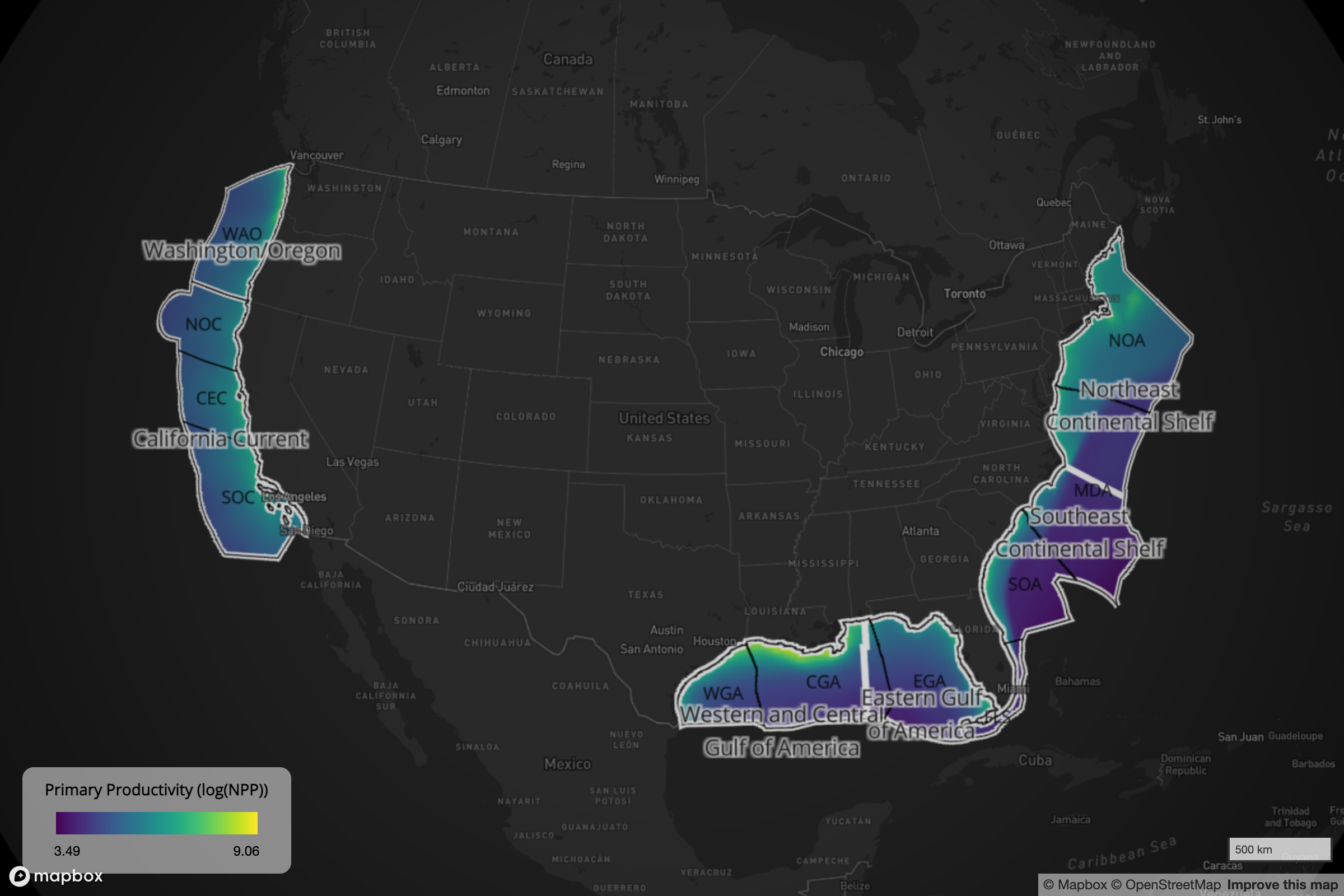
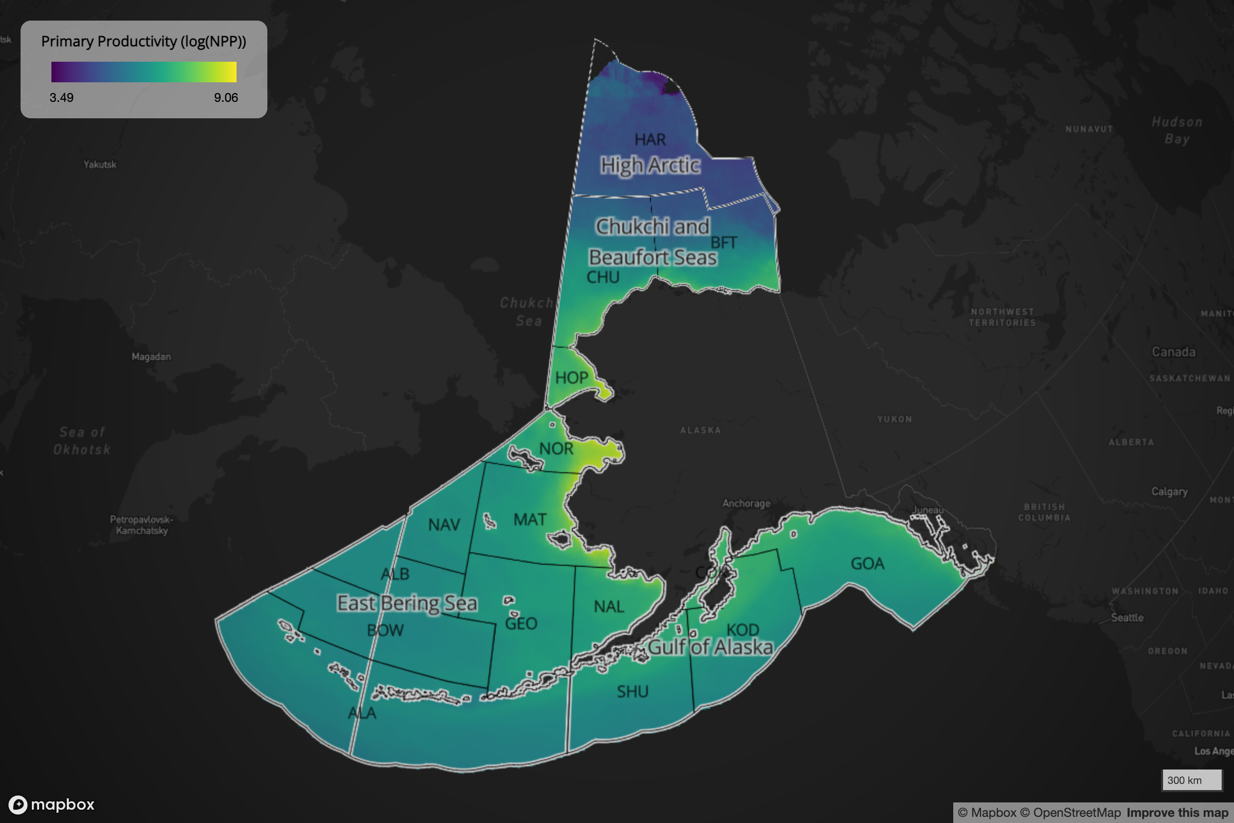
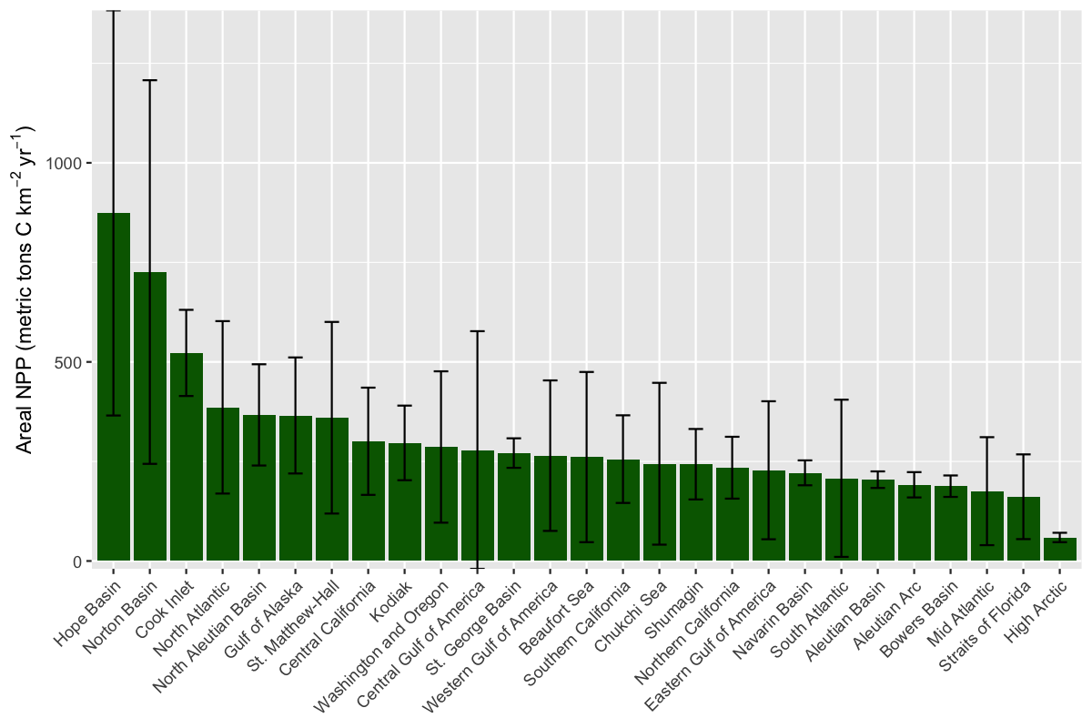
Primary Productivity
Net Primary Productivity (NPP) was calculated using the Vertically Generalized Production Model (VGPM) (Behrenfeld and Falkowski 1997) with VIIRS satellite data (R2022 version) for the most recently completed decade (2014 to 2023). The VGPM is a chlorophyll-based model that estimates net primary production using a temperature-dependent description of chlorophyll-specific photosynthetic efficiency. Monthly NPP data at 0.083° resolution (2160×4320 global grid) were downloaded from Oregon State University’s Ocean Productivity website as HDF files, processed to extract NPP values (units: mg C m-2 day-1), and averaged annually for each year. The 10-year mean and standard deviation were then calculated across all years. The high-resolution productivity raster was downsampled to match the 0.05° species distribution grid using bilinear interpolation and masked to the study area. For Planning Area summaries, zonal statistics were computed using area-weighted means, and values were converted to metric tons C km-2 yr-1 for easier interpretation.
Spatial Aggregation and Rescaling
Scores from individual grid cells are aggregated to BOEM Planning Areas through a multi-step process that ensures ecologically meaningful comparisons across diverse marine regions.
Step 1: Cell-level scoring. For each 0.05° grid cell, the raw vulnerability score (\(v_c\)) is calculated by summing the products of species presence (\(p_{sc}\)) and extinction risk weight (\(w_s\)) across all species in a taxonomic group, as described above.
Step 2: Ecoregional rescaling. Raw cell scores are rescaled to a 0-100 range within each BOEM Ecoregion. This normalization accounts for natural differences in species richness between regions. For example, the species-rich Gulf of America naturally produces higher raw scores than the Arctic; rescaling ensures that a score of 80 in the Gulf of America and a score of 80 in the Arctic both represent similarly high relative sensitivity within their respective ecological contexts. The rescaling formula for each cell is:
\[
v_{c,rescaled} = \frac{v_c - v_{min,ecoregion}}{v_{max,ecoregion} - v_{min,ecoregion}} \times 100
\]
Step 3: Planning Area aggregation. Rescaled cell scores are aggregated to Planning Areas using area-weighted averages. Each cell’s contribution is proportional to the fraction of its area that falls within the Planning Area. This ensures that larger cells at lower latitudes do not disproportionately influence scores relative to smaller cells at higher latitudes.
Worked example. Consider a simplified Planning Area containing three cells in the Western Central Ecoregion, where the ecoregion minimum fish score is 65 and the maximum is 974:
| A |
200 |
(200-65)/(974-65)×100 = 15 |
25 |
0.33 |
| B |
600 |
(600-65)/(974-65)×100 = 59 |
25 |
0.33 |
| C |
400 |
(400-65)/(974-65)×100 = 37 |
25 |
0.33 |
The Planning Area fish score = (15×0.33 + 59×0.33 + 37×0.33) = 37. This value can be directly compared with fish scores from Planning Areas in other ecoregions.
BOEM Ecoregions used for rescaling are defined in Geographic Scope below.
Data Quality Control and Validation
Multiple quality control procedures ensure data integrity and biological realism:
Spatial Validation: All species distributions were validated against independent occurrence data from OBIS (Ocean Biodiversity Information System) and GBIF. Distributions showing implausible ranges (e.g., Pacific Walrus presence in Atlantic waters due to outdated AquaMaps historical extents) were corrected by masking AquaMaps distributions to IUCN RedList global range maps, ensuring model outputs reflect present-day species ranges. Additional validation used temporal occurrence filters (10, 20, and 50-year windows) and expert review.
Taxonomic Reconciliation: Duplicate species records arising from taxonomic synonyms were resolved using ordered taxonomicStatus factors (accepted > unassessed > unaccepted). For WoRMS matches with multiple candidate taxa (n=270 species with 2-9 matches each), the accepted name was preferentially selected. Species with conflicting classifications across authorities were manually reviewed.
Range Map Realism: Critical habitat and range map polygons were validated for geometric validity (st_make_valid()) and topological errors. Rasterization artifacts (e.g., slivers < 2 km²) were reassigned to the dominant ecoregion. Anti-meridian crossing geometries were corrected using st_shift_longitude() and st_wrap_dateline() transformations.
Presence Value Calibration: Continuous suitability models (AquaMaps: 0-100%) were used directly, while binary range maps were assigned presence values reflecting data quality: Critical Habitat (70-90%) reflects high-quality, legally-designated areas; expert range maps (50%) reflects broader, less certain extents following IUCN Species Information Service conventions.
Temporal Currency: Primary productivity data (2014-2023) and species assessments (most recent IUCN evaluation) ensure temporal consistency. Historic distributions were corrected by masking to IUCN global range maps where contemporary evidence indicated that modeled ranges did not reflect current species distributions.
Geographic Scope
The MST uses BOEM Ecoregions as its primary geographic units. These ecoregions are defined by Large Marine Ecosystem boundaries, bathymetry, hydrography, productivity, and species composition (Morandi et al. 2018); the High Arctic Planning Area is treated as its own dedicated ecoregion. The analysis is conducted at a 0.05° grid resolution (6,224,618 cells after masking to study area), providing detailed coverage across U.S. waters and spanning Arctic, temperate, and subtropical marine ecosystems.
Species distributions were ingested for the full set of 36 OCS Planning Areas spanning the lower 48 states, Alaska, and U.S. Pacific Island territories. The descriptive maps and flower plots in this report (Figure 5 through Figure 9) summarize only the 27 BOEM Planning Areas in the continental U.S. and Alaska (19 in lower 48 states, 8 in Alaska); the interactive applications (Figure 10 through Figure 13) expose the full territorial extent.
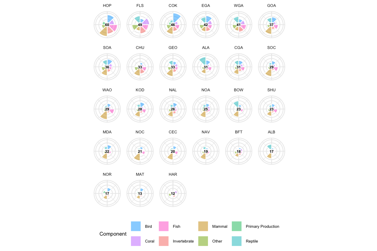
Visualization and Decision Support
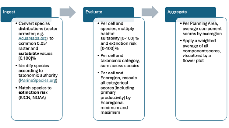
The MST utilizes interactive visualizations, including the Flower Plot (see Figure 9 and the interactive app), to convey complex vulnerability assessment results. The Flower Plot displays component sensitivity scores for each Planning Area, where:
Each petal represents a taxonomic group (e.g., mammals, birds, fish, invertebrates, corals, turtles) or primary productivity. The length of the petal reflects the rescaled sensitivity score (0-100) for that component within the Planning Area.
The center number is the overall composite sensitivity score, calculated as the equal-weighted average of all component scores.
For example, a Planning Area with a long mammal petal and short fish petal indicates relatively high marine mammal sensitivity but lower fish sensitivity. This decomposition helps decision-makers identify which ecological elements are driving vulnerability in a given location, supporting more informed spatial planning and targeted impact assessment.
Results
Maps of Environmental Sensitivity by Pixel
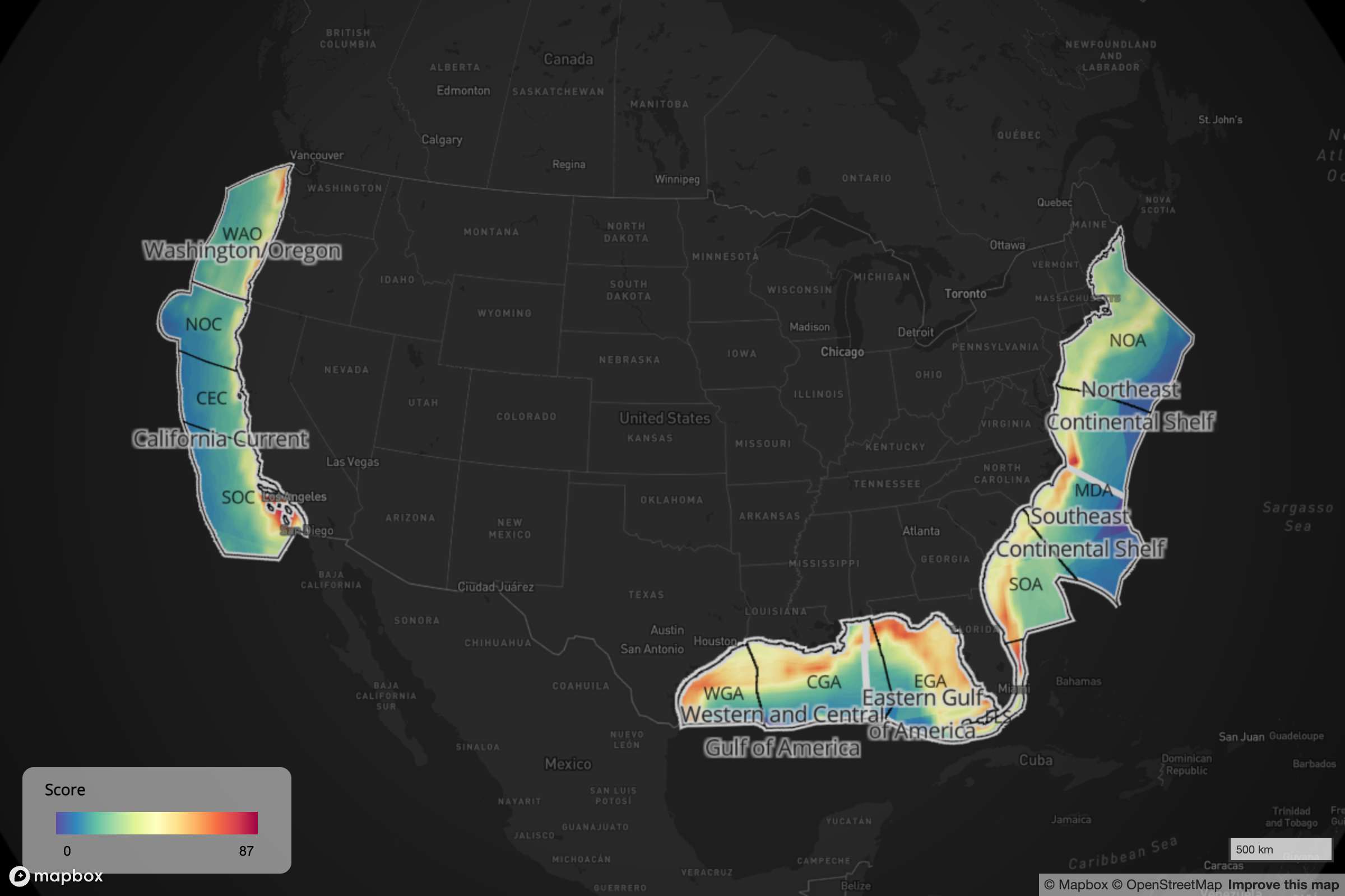
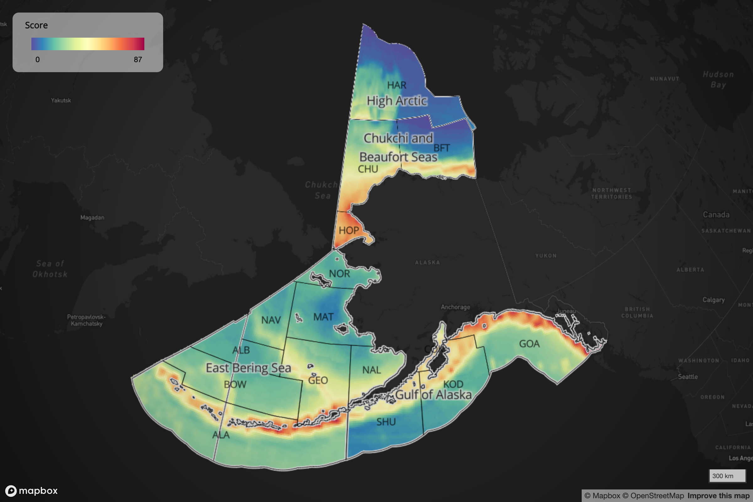
Pixel-level maps reveal the fine-scale spatial pattern of environmental sensitivity across U.S. waters at the native 0.05° (~5 km) cell resolution. In the contiguous U.S. (Figure 5), the highest sensitivity scores concentrate along the productive shelf edges and biodiversity-rich subtropical waters of the Gulf of America, the Atlantic Bight, and the California Current. In Alaska (Figure 6), the highest scores fall along the productive Bering Sea and Aleutian shelves, while the cold High Arctic shows characteristically lower raw species richness. Within-ecoregion rescaling preserves these regional contrasts while still allowing cell-level differentiation of localized hotspots.
Maps of Environmental Sensitivity by Planning Area
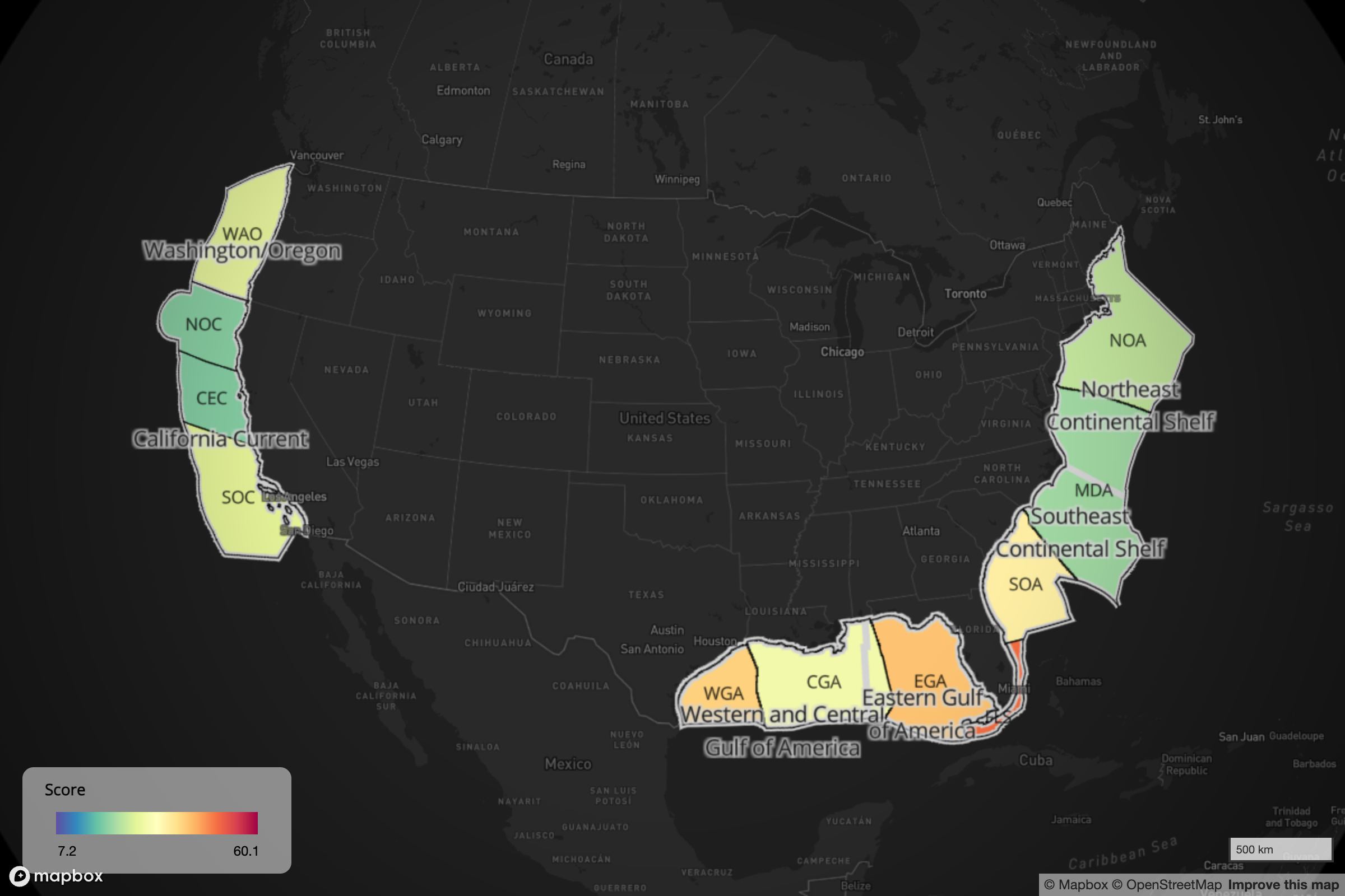
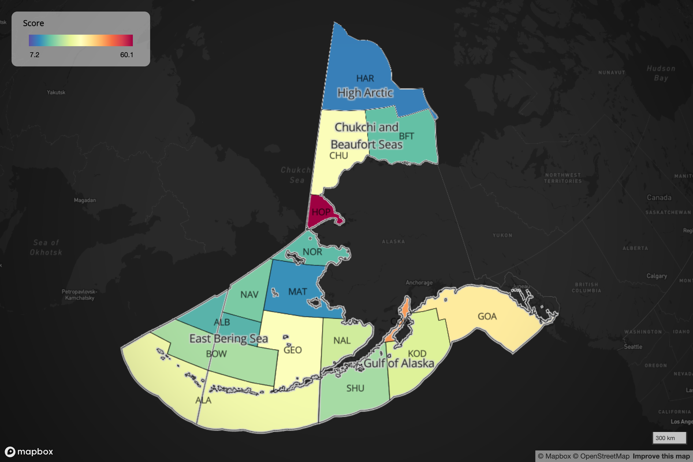
Pixel scores aggregated to Planning Area boundaries (Figure 7, Figure 8) provide the management-relevant unit for BOEM leasing decisions. Aggregation uses the area-weighted mean of rescaled cell scores within each Planning Area, so larger Planning Areas do not automatically score higher than small ones. The aggregated view smooths cell-level noise and surfaces between-Planning-Area comparisons, while the pixel maps above retain the within-Planning-Area heterogeneity needed for site-specific stipulations.
Flower Plot Scores of Environmental Sensitivity by Planning Area
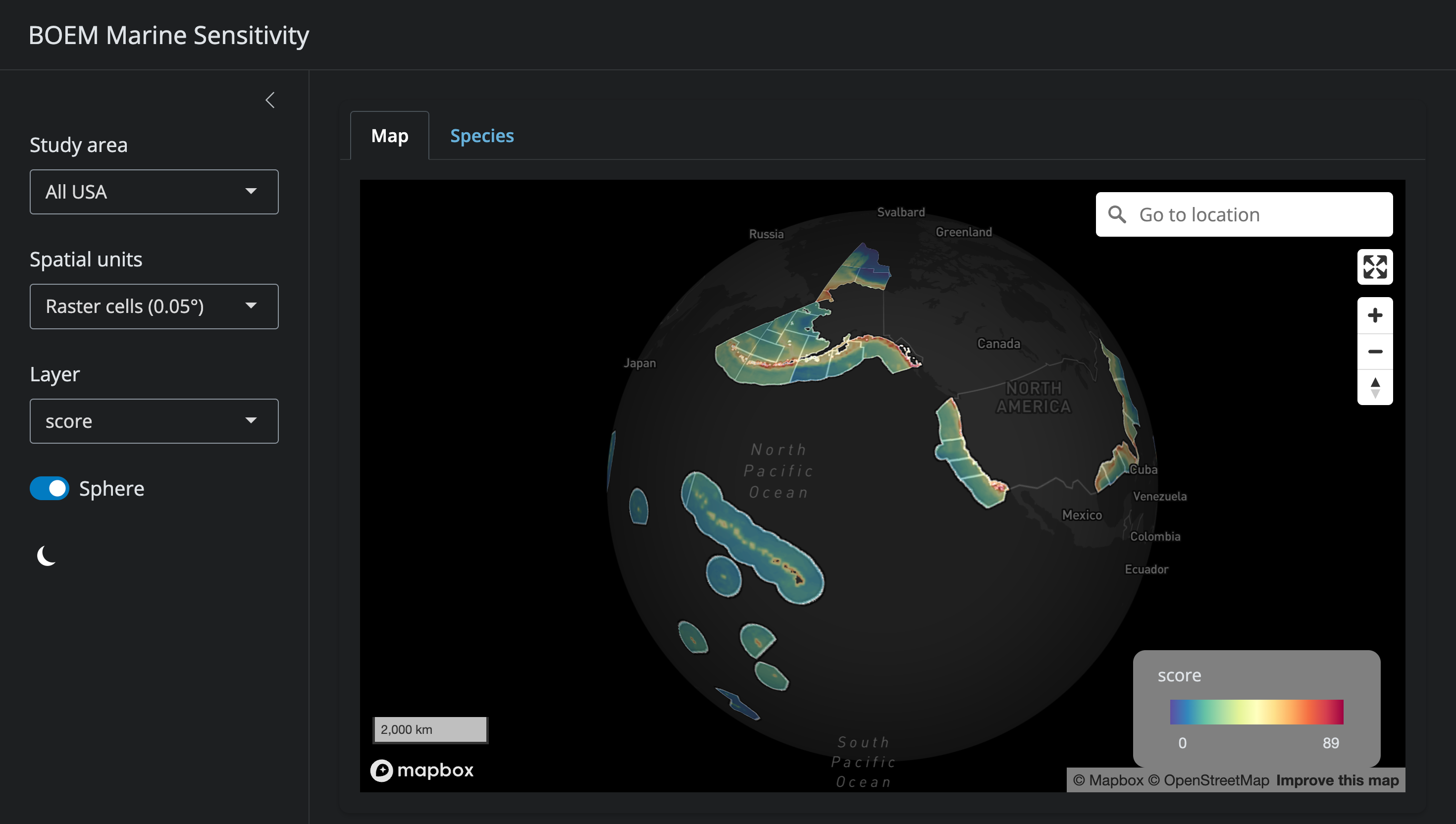
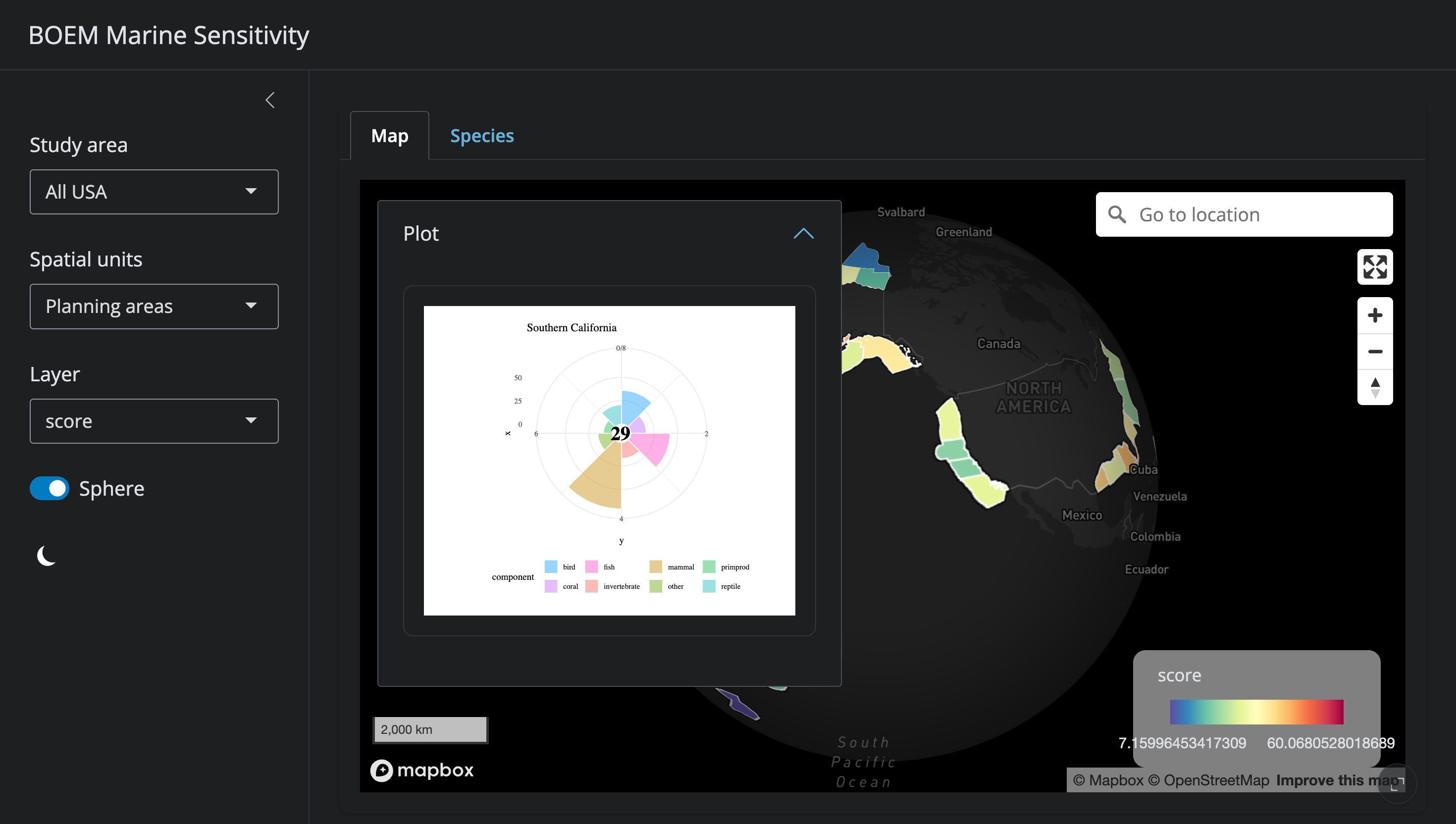
Online Mapping Application
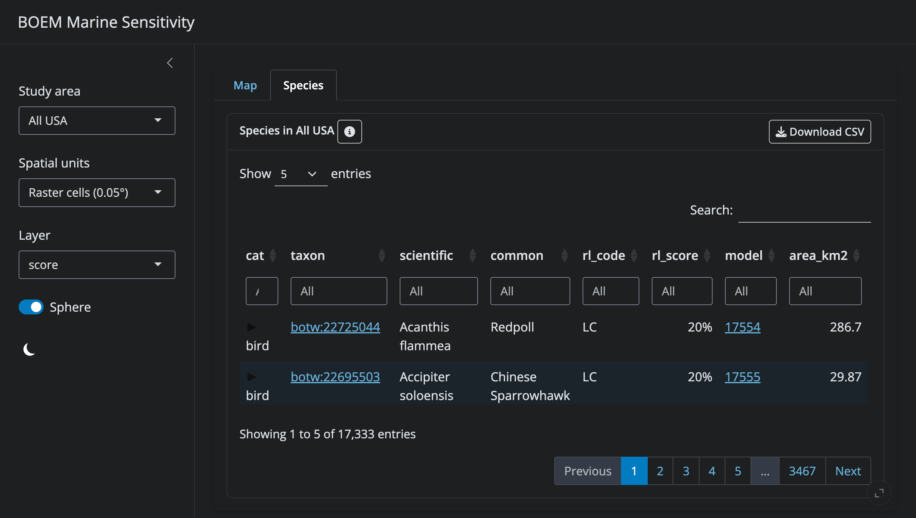
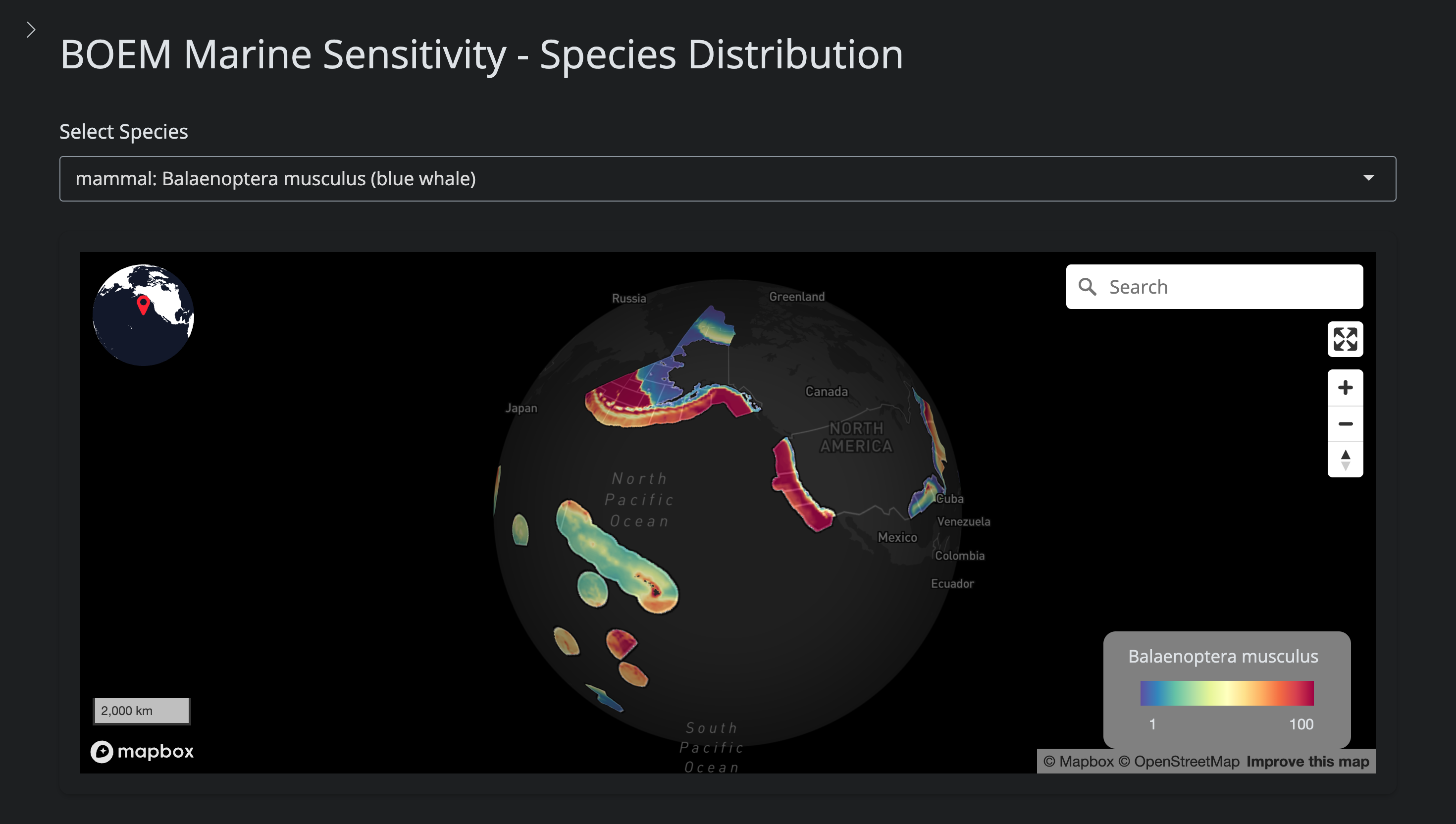
The MST includes an interactive web application that allows users to explore sensitivity scores across Planning Areas, taxonomic groups, and individual species. Users can switch between pixel- and Planning-Area-level views, filter by component (e.g. fish, birds, mammals, productivity), hover for cell-level values, click any Planning Area to open its flower plot, and click any species in the Species table to drill into a per-species distribution map. The application is built on cloud-native vector and raster tile services and exposes the full territorial extent (all 36 Planning Areas), complementing the static maps in this report.
The main app mapgl app (Figure 10; Figure 11; Figure 12) shows the overall scores and any underlying components by 0.05° raster cell or Planning Area, all masked by the chosen Study area. The model link in the Species table (Figure 12) links to the species distribution app mapsp (Figure 13), which shows the distribution of the species, in this case for the blue whale, which is globally distributed.
Reproducible Infrastructure
The MST is built entirely using open-source tools, and all source code is publicly available through GitHub at github.com/MarineSensitivity. The entire workflow, from data acquisition to sensitivity scoring, is documented in executable Quarto notebooks and available for independent review and replication. This commitment to transparency ensures that the analysis can be verified, updated, and extended as new data becomes available or methodologies evolve.
The MST comprises 8 core infrastructure components, each maintained as a separate GitHub repository. These tools and analyses are works in progress and will be continually updated as new data and methods become available.
Server
Server
All server software is set up using containerized open-source components with Docker, so the full stack can be rebuilt with a single docker compose up and handed off to BOEM for internal hosting. Containerized services include Shiny (interactive apps), RStudio (analyst environment), R Plumber (custom API), PostGIS (spatial database), Caddy (reverse proxy with automatic TLS), pg_tileserv (vector tile server), and TiTiler (raster tile server). This containerized approach ensures reproducibility across machines and simplifies disaster recovery.
Database
A spatially enabled PostgreSQL/PostGIS database serves the vector data (Planning Areas, Ecoregions, species range polygons) for transactional access from the apps and tile services. It is complemented by DuckDB, an embedded columnar analytical engine with spatial extensions, which holds the species × cell × metric tables used to generate biodiversity rasters on the fly. The split lets transactional vector reads remain fast while enabling SQL analytics over hundreds of millions of cell × species rows from a single file. The current production DuckDB footprint is roughly 2 GB; backups run nightly to a separate volume.
Workflows
Workflows
The scientific workflows are a collection of Quarto notebooks (R and Python) that perform data acquisition, ingestion, validation, and derived-product generation. Each notebook is rendered to HTML for inspection and archived alongside its source so that every intermediate decision (taxonomic mappings, masking rules, threshold choices) is reviewable. Representative notebooks include ingest_aquamaps_to_sdm_duckdb.qmd (downscaling AquaMaps to 0.05°), ingest_birdlife.org_botw.qmd (rasterizing BirdLife range maps), ingest_productivity.qmd (VGPM annual productivity averages), merge_models.qmd (taxonomically reconciling overlapping species), and calc_scores.qmd (cell- and Planning-Area-level scoring). The notebooks form a directed pipeline from raw data to the database tables underpinning the apps and reports.
Libraries
Libraries
Packaging functions with documentation enables reusability across analysis and visualization for simplifying existing applications while extending functionality to outside projects. The msens R package provides functions for analyzing biodiversity data on the desktop.
Docs
Docs
The documentation is principally a book (rendered from Quarto) oriented for scientific and technical audiences, but also applies to documentation throughout the project for reproducibility and usability.
Website
Website
The website marinesensitivity.org provides the project landing page with the general public as the initial audience, with content and links (such as to the docs) for deeper understanding.
Conclusions
The Marine Sensitivity Toolkit represents a transformative advancement in BOEM’s capability to fulfill its statutory mandate under the Outer Continental Shelf Lands Act. By integrating 17,333 species distribution models, comprehensive extinction risk data, and decade-averaged primary productivity across 6.2 million high-resolution grid cells, the MST delivers unprecedented spatial detail and taxonomic coverage for environmental decision-making. This v1 deliverable establishes the foundational framework and analytical infrastructure; the MST will be continually refined as new data sources, improved species distribution models, and enhanced methodologies become available.
Alignment with FAIR Data Principles
The MST fully embodies FAIR (Findable, Accessible, Interoperable, Reusable) data principles, ensuring long-term utility and scientific integrity:
Findable: All data products, code repositories, and documentation are indexed through persistent URLs at marinesensitivity.org with comprehensive metadata. Species distributions are linked to authoritative taxonomic identifiers (WoRMS AphiaID, GBIF taxonID, ITIS TSN, IUCN taxon ID), enabling unambiguous species lookup across databases. DOIs will be assigned to major data releases for permanent scholarly citation.
Accessible: Interactive web applications (https://app.marinesensitivity.org/mapgl_v1) provide immediate public access to sensitivity scores and underlying data without requiring specialized software. Programmatic access through RESTful APIs (tile.marinesensitivity.org, api.marinesensitivity.org) enables automated data retrieval for research and operational applications. All source code is publicly available through GitHub under open-source licenses.
Interoperable: Data products adhere to Open Geospatial Consortium (OGC) standards including GeoTIFF, GeoJSON, and vector tiles. DuckDB analytical database enables SQL-based querying with spatial extensions. Future deployment of STAC (SpatioTemporal Asset Catalog) catalogs will enable seamless integration with cloud-native geospatial workflows. Species taxonomies are cross-referenced to ensure interoperability with OBIS, GBIF, IUCN, and other biodiversity platforms.
Reusable: Complete analytical workflows are documented in executable Quarto notebooks (e.g., ingest_aquamaps_to_sdm_duckdb.qmd, ingest_productivity.qmd, calc_scores.qmd) with explicit provenance from raw data to final products. Modular R packages (msens) provide reusable functions for sensitivity analysis beyond BOEM applications. Comprehensive metadata describe data quality, uncertainty, and appropriate use limitations.
Meeting Executive Order 14303 Requirements
In direct response to Executive Order 14303: Restoring Gold Standard Science (May 29, 2025), the MST exemplifies scientific integrity through:
Best Available Science: Integration of the most current, peer-reviewed data sources including AquaMaps 2019, BirdLife BOTW 2024.2, IUCN Red List 2025, and VIIRS-VGPM 2023. Regular update cycles ensure incorporation of new species assessments, range shifts, and improved distribution models.
Transparency: Every analytical step is documented with source code and intermediate outputs publicly accessible. Sensitivity scoring algorithms are mathematically explicit with clear justification for weighting schemes. Quality control procedures are documented, including handling of data conflicts and uncertainty.
Reproducibility: Complete computational environment specified through Docker containers and R package versions. Workflows use directed acyclic graphs (DAGs) to track data dependencies, ensuring any component can be regenerated from source data. Version control through GitHub enables tracking of methodological evolution.
Peer Review: Methods build upon established ecological risk assessment frameworks (e.g., IUCN spatial data standards, VGPM productivity model validation literature) with transparent adaptation for BOEM’s decision context.
Rapid Species-at-Risk Assessment
The MST provides unprecedented capability for rapid identification and characterization of species at elevated risk within proposed lease areas:
Fine-Scale Spatial Resolution: The 0.05° grid captures habitat heterogeneity and localized species hotspots often missed by coarser assessments, enabling differentiation of sensitivity within Planning Areas to support site-specific lease stipulations.
Taxonomic Comprehensiveness: Coverage of 17,333 species across all major marine taxa (6,672 fishes, 8,179 invertebrates, 460 birds, 775 corals, 88 mammals, 31 turtles, plus 1,128 other marine taxa) ensures no major taxonomic group is overlooked. Subsequent post-v1 development has integrated NMFS Critical Habitat, U.S. Fish and Wildlife Service Critical Habitat, and FWS Current Range Maps to provide direct linkage to ESA-listed species protections in the next release.
Extinction Risk Integration: Direct linkage of species distributions to IUCN Red List and ESA status enables immediate identification of threatened and endangered species within any area of interest. The precautionary principle (using maximum risk category when multiple assessments exist) ensures conservative risk characterization.
Dynamic Query Capability: Interactive applications enable real-time exploration of sensitivity drivers. Users can identify which specific species, taxonomic groups, or risk categories contribute most to a location’s sensitivity score, facilitating targeted impact assessment and mitigation design.
Ecoregional Context: Rescaling within ecoregions provides ecologically meaningful comparisons. A “moderate” sensitivity score in the species-rich Gulf of America represents fundamentally different ecological conditions than the same score in the Arctic, enabling region-appropriate decision-making.
Foundation for Mitigation and Adaptive Management
Sensitivity scores directly inform multiple stages of offshore energy development planning and mitigation:
Lease Area Identification: High-resolution sensitivity maps (Figure 5, Figure 6) provide a full spectrum of sensitivity across U.S. waters, from low to high. Areas with lower sensitivity scores represent locations where offshore energy development may proceed with reduced ecological risk, making them strong candidates for priority leasing consideration. Conversely, areas with higher sensitivity scores indicate biodiversity hotspots and endangered species habitat where enhanced protections may be warranted. Flower plots (Figure 9) reveal which taxonomic groups drive sensitivity in each Planning Area, enabling targeted avoidance strategies focused on the most ecologically significant components.
Temporal Restrictions: Integration of seasonal species distribution models (future Phase 2 enhancement) will support temporal lease stipulations (e.g., avoiding construction during seabird breeding seasons, marine mammal calving periods, or sea turtle nesting migrations).
Site-Specific Stipulations: Cell-level sensitivity scores enable graduated mitigation requirements scaled to local ecological importance. Areas with CR (Critically Endangered) species presence may require enhanced monitoring, operational restrictions, or exclusion zones beyond standard best management practices.
Cumulative Impact Assessment: Standardized sensitivity metrics enable quantitative evaluation of cumulative effects across multiple projects. Summing impacted cell scores provides objective basis for determining when cumulative thresholds warrant enhanced mitigation or alternative analysis.
Adaptive Management Triggers: Baseline sensitivity characterization establishes quantitative monitoring targets. Post-construction monitoring can assess whether observed impacts remain within predicted sensitivity envelopes, triggering adaptive management when thresholds are exceeded.
Mitigation Hierarchy Application: The MST supports systematic application of the mitigation hierarchy (avoid > minimize > restore > offset). High sensitivity areas inform avoidance strategies. Moderate sensitivity areas guide minimization measures. Quantified sensitivity losses inform compensatory mitigation scaling.
Scientific and Policy Implications
The MST methodology is readily transferable to other ocean planning contexts including marine protected area design, essential fish habitat designation, shipping route optimization, and marine spatial planning. The open-source, cloud-native architecture enables adoption by other agencies and nations with minimal technical barriers. As species distribution models improve, extinction risk assessments update, and new data sources emerge, the MST provides a stable framework for incorporating best available science into iterative planning cycles, fully realizing the vision of Executive Order 14303 for transparent, reproducible, science-based environmental decision-making.
Next Steps
The MST is designed to be a living system that will be continually updated as new data becomes available and methodologies evolve. In Phase 2, planned enhancements include:
Refining species distribution models by validating AquaMaps distributions against contemporary occurrence data from OBIS and GBIF, and continuing to constrain ranges using IUCN spatial range maps.
Refining regulatory and listed-species coverage by maintaining up-to-date integration of NMFS Critical Habitat, FWS Critical Habitat, and FWS Current Range Maps as new designations and assessments are issued.
Enhancing geospatial infrastructure by exporting biodiversity metrics to cloud-optimized GeoTIFFs (COGs) organized in spatio-temporal asset catalogs (STACs) for faster rendering and broader reuse.
Expanding the interactive applications to support arbitrary area selection (drawn polygons, uploaded shapefiles, gazetteer identifiers) and taxonomic tree navigation for merged products.
Improving data products and delivery by documenting functions into the msens R library, implementing a directed acyclic graph (DAG) data pipeline using the targets library, and providing outputs in multiple formats (shapefile, GeoPackage, GeoJSON, GeoTIFF, COG).
Automating high-quality figure generation including vector graphics suitable for publication and interactive story-map explainers.
Transferring data and tools to BOEM servers to ensure all code and data are entirely maintainable internally.
All code will continue to be stored in publicly accessible GitHub repositories under github.com/MarineSensitivity, with version tags corresponding to each model iteration.
Study Products
The following products were delivered as part of this study:
Map of Study Area
The study area encompasses the 27 BOEM OCS Planning Areas in the contiguous U.S. and Alaska (19 in the lower 48, 8 in Alaska), spanning Arctic, temperate, and subtropical marine ecosystems across U.S. federal waters. BOEM Planning Areas are used as the primary unit because they are the operational geography for OCS leasing and stipulation decisions, ensuring that sensitivity outputs map directly onto BOEM’s decision contexts. Anti-meridian crossing for the western Aleutians and U.S. Pacific Island territories was handled with st_shift_longitude() and st_wrap_dateline() so that all spatial joins, area calculations, and rasterizations remain valid across the dateline. Maps of the study area showing environmental sensitivity scores by pixel and by Planning Area are presented in Figure 5, Figure 6, Figure 7, and Figure 8.
10 References
Behrenfeld, Michael J, and Paul G Falkowski. 1997. “Photosynthetic Rates Derived from Satellite-Based Chlorophyll Concentration.” Limnology and Oceanography 42 (1): 1–20.
Elith, J., and J. Leathwick. 2009. “Conservation Prioritisation Using Species Distribution Modelling.” Spatial Conservation Prioritization: Quantitative Methods and Computational Tools, 70–93.
Morandi, A., S. Berkman, J. Rowe, R. Balouskus, D. S. Etkin, C. Moelter, and D. Reich. 2018.
“Environmental Sensitivity and Associated Risk to Habitats and Species on the Pacific West Coast and Hawaii with Offshore Floating Wind Technologies.” OCS Study BOEM 2018-031.
Camarillo, CA:
US Department of the Interior, Bureau of Ocean Energy Management, Pacific OCS Region.
https://www.boem.gov/sites/default/files/environmental-stewardship/Environmental-Studies/Pacific-Region/Studies/BOEM-2018-031-Vol1.pdf.
Niedoroda, A, S Davis, M Bowen, E Nestler, J Rowe, R Balouskus, M Schroeder, B Gallaway, and R Fechhelm. 2014. “A Method for the Evaluation of the Relative Environmental Sensitivity and Marine Productivity of the Outer Continental Shelf.”