            Bairds         BLUE WHALE       BRYDES WHALE       BTLN Coastal
               810                810                810                162
     CA N FUR SEAL        CA Sea Lion   CAmerDPSHUMPBACK     DALLS PORPOISE
               810                810                810                810
      ENP FUR SEAL     ENP GRAY WHALE          FIN WHALE              GREEN
               810                810                810                810
GUADALUPE FUR SEAL       Harbor OR WA    HARBOR PORPOISE     Harbor Seal CA
               810                810                342                810
   HI DPS_HUMPBACK         K WHALE OS        K WHALE Res         K WHALE Tr
               810                810                810                810
          Lags WSD            LB COMN        LEATHERBACK          Liso NRWD
               810                810                810                810
        LOGGERHEAD    MexDPS_HUMPBACK        MINKE WHALE           N E Seal
               810                810                810                810
      OLIVE RIDLEY      PYGMY & DWARF        RIGHT WHALE              Risso
               810                810                810                810
   S-F PILOT WHALE            SB COMN          SEI WHALE        SPERM WHALE
               810                810                810                810
  STELLER SEA LION     WNP GRAY WHALE Ziphius-Mesoplodon
               810                810                810
4.3 Counts of factor
Code
table(d$factor, useNA ="ifany")
                  1. Population Factors 2. Species Habitat and Temporal Factors
                                   6772                                    5079
        3. Physical Interaction Factors              4. Other Stressors Factors
                                   6772                                    6772
                                    ALL
                                   5079
4.4 Counts of factor_element
Code
table(d$factor_element, useNA ="ifany")
                         1. Population Factors: Pop. Size
                                                     1693
                       1. Population Factors: Pop. Status
                                                     1693
                        1. Population Factors: Pop. Trend
                                                     1693
                          1. Population Factors: subtotal
                                                     1693
     2. Species Habitat and Temporal Factors: Habitat Use
                                                     1693
        2. Species Habitat and Temporal Factors: subtotal
                                                     1693
2. Species Habitat and Temporal Factors: Temporal Overlap
                                                     1693
            3. Physical Interaction Factors: Entanglement
                                                     1693
                 3. Physical Interaction Factors: Masking
                                                     1513
 3. Physical Interaction Factors: Masking/Electromagnetic
                                                      180
                3. Physical Interaction Factors: subtotal
                                                     1693
           3. Physical Interaction Factors: Vessel Strike
                                                     1693
          4. Other Stressors Factors: Chronic anth. noise
                                                     1693
          4. Other Stressors Factors: Chronic anth. other
                                                     1693
      4. Other Stressors Factors: Chronic biological risk
                                                     1693
                     4. Other Stressors Factors: subtotal
                                                     1693
                                    ALL: CONFIDENCE LEVEL
                                                     1693
                                               ALL: TOTAL
                                                     1693
                                ALL: VULNERABILITY RATING
                                                     1693
References
Southall, Brandon, Robert Mazurek, and Rikki Eriksen. 2023. “Vulnerability Index to Scale Effects of Offshore Renewable Energy on Marine Mammals and Sea Turtles Off the U.S. West Coast (VIMMS).” OCS Study BOEM 2023-057. Camarillo (CA): U.S. Department of the Interior, Bureau of Ocean Energy Management.
Source Code
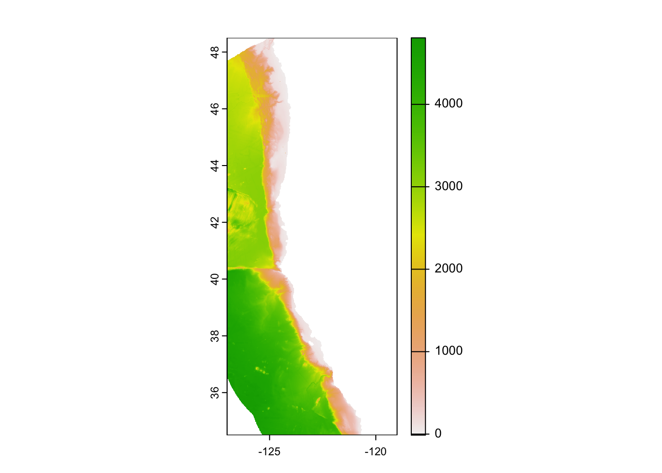
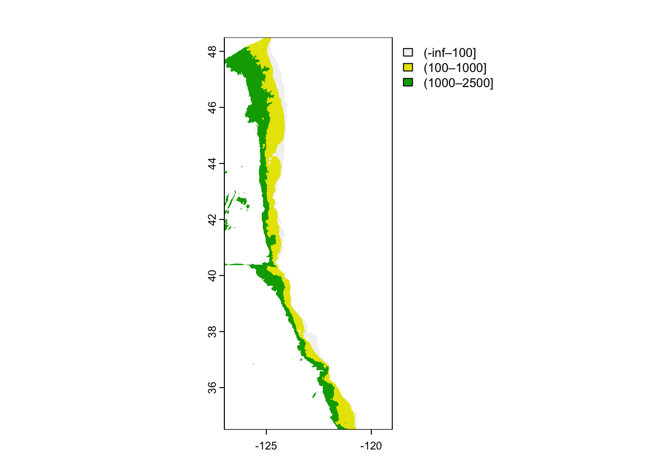
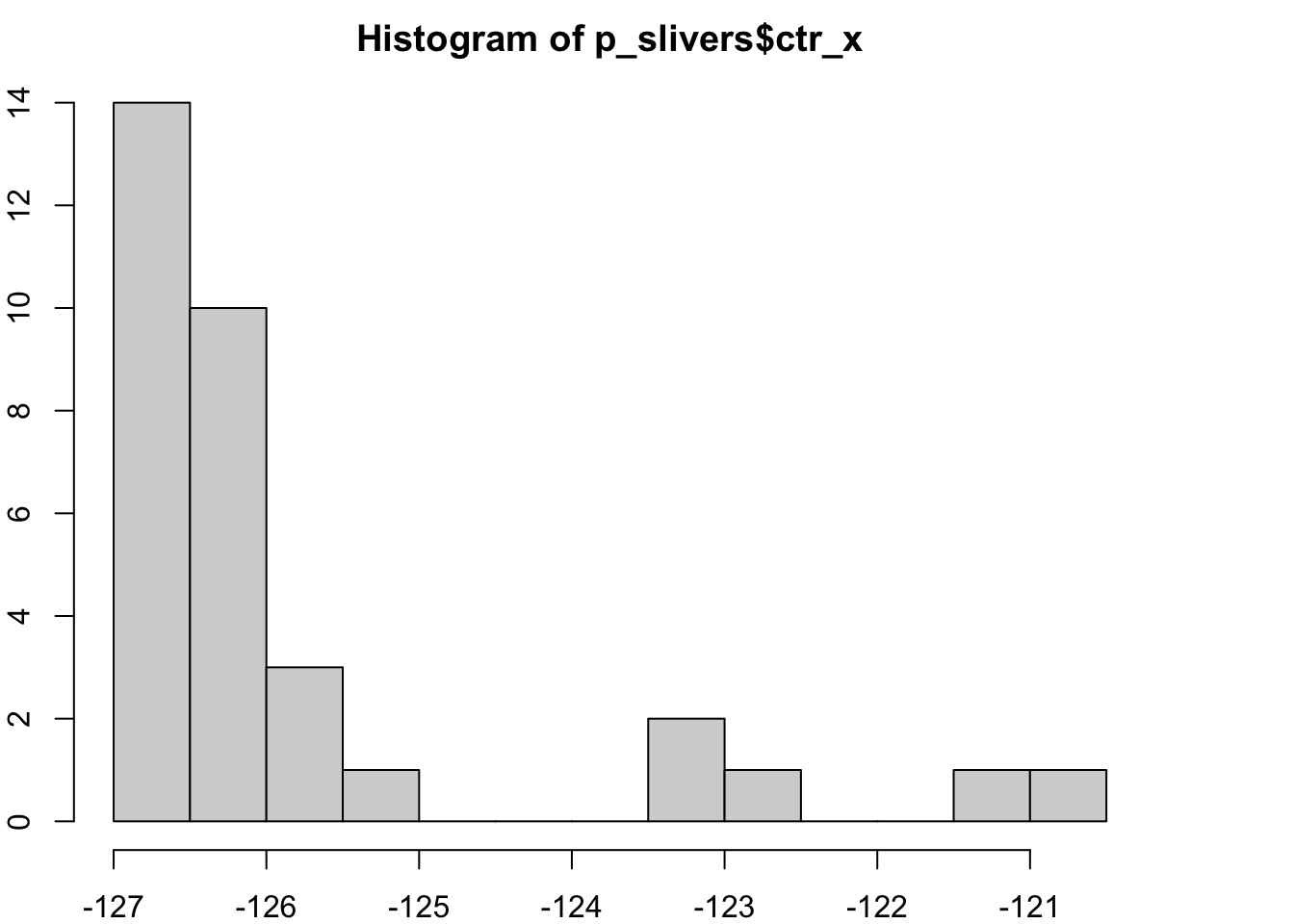
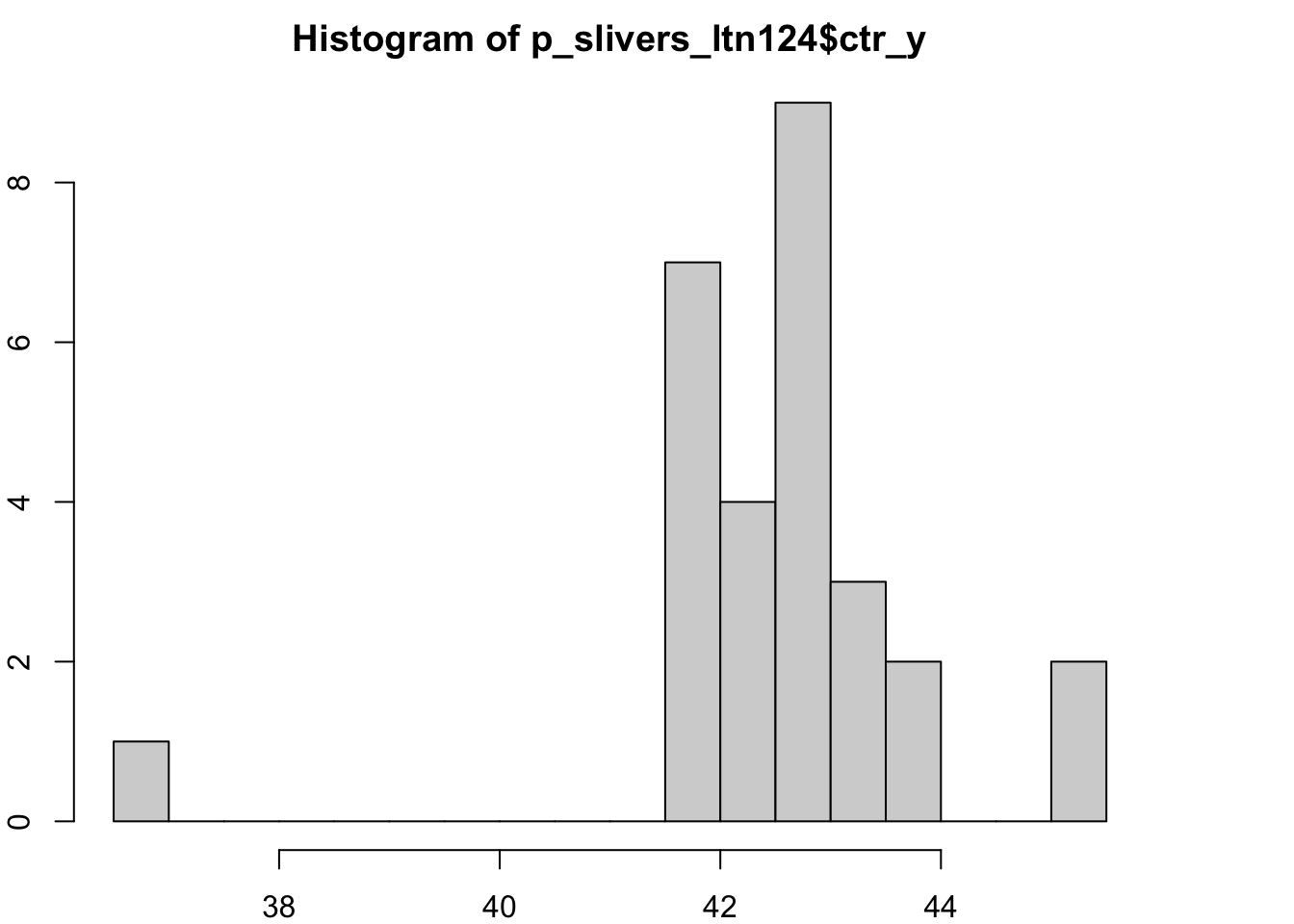
---title: "Explore Species Sensitivities (Southall et al, 2023)"editor_options: chunk_output_type: consoleformat: html: css: ./libs/leaflet-control.css---## IntroductionThis report by Southall et al. [-@southallVulnerabilityIndexScale2023] describes species vulnerability based on multiple criteria:- **Space** - Latitudinal zones - `Zone 1`\ Central California\ 34.5° N to 38.33° N - `Zone 2`\ Northern California\ 38.33° N to 42° N - `Zone 3`\ Southern and Central Oregon\ 42° N to 45° N - `Zone 4`\ Columbia River Region\ 45° N to 47.1° N - `Zone 5`\ Central and Northern Washington (Offshore)\ 47.1° N to 48.5° N - Depth regimes - `Shelf`\\< 100 m - `Slope`\ 100-1,000 m - `Oceanic`\ 1,000 - 2,500 m- **Time**\ Oceanographic season - `Upwelling`\ March--June - `Post Upwelling`\ July--November - `Winter`\ December--February- **Taxa**\ including sub-population or stock.## Space```{r}#| label: setup#| warning: falselibrarian::shelf( dplyr, DT, fs, glue, here, knitr, leaflet, mapview, MarineSensitivity/msens, purrr, readr, readxl, sf, stringr, terra, tibble, tidyr, units,quiet = T)show_all <- Tdir_data <-"/Users/bbest/My Drive/projects/msens/data"g_tif <-glue("{dir_data}/derived/gebco_depth.tif")p_geo <-here("data/Southall-2023_depth-regimes.geojson")dir_xlsx <-glue("{dir_data}/raw/studies/southallVulnerabilityIndexScale2023")vuln_csv <-here("data/Southall-2023_vulnerabilities.csv")``````{r}#| label: space#| warning: falseif (!file.exists(p_geo) | show_all){ bbox <-c(-127+360, -119+360, 34.5, 48.5) # (xmin, xmax, ymin, ymax) r_g <-rast(g_tif, win=bbox)ext(r_g) <- bbox -c(360,360,0,0)plot(r_g)# apply focal window to smooth out the raster r_gf <-focal(r_g, w=5, fun="mean", na.rm=T)names(r_gf) <-"depth"# classify into depth regimes r_gc <-classify(r_gf, c(-Inf, 100, 1000, 2500))plot(r_gc)# convert to polygons, calculate area, # and centroid for filtering slivers p <-as.polygons(r_gc) |>st_as_sf() |>st_cast("POLYGON") |>mutate(ctr_x =st_centroid(geometry) |>st_coordinates() %>% .[,1],ctr_y =st_centroid(geometry) |>st_coordinates() %>% .[,2],area_km2 =st_area(geometry) |>set_units(km^2) |>as.numeric())# table(p$depth) # before focal()# (-inf–100] (100–1000] (1000–2500] # 137 133 192 # table(p$depth) # w=3# (-inf–100] (100–1000] (1000–2500] # 44 47 61 # table(p$depth) # w=5# (-inf–100] (100–1000] (1000–2500] # 36 24 34 p_deep = p |>filter( depth =="(1000–2500]", area_km2 >1000) p_other = p |>filter( depth !="(1000–2500]") p_slivers <- p |>filter( depth =="(1000–2500]", area_km2 <1000)hist(p_slivers$ctr_x, breaks=20) p_slivers_gtn122 <- p |>filter( depth =="(1000–2500]", area_km2 <1000, ctr_x >-122) # keep p_slivers_ltn122gt124 <- p |>filter( depth =="(1000–2500]", area_km2 <1000, ctr_x <-122, ctr_x >-124) # keep p_slivers_ltn124 <- p |>filter( depth =="(1000–2500]", area_km2 <1000, ctr_x <-124) # removehist(p_slivers_ltn124$ctr_y, breaks=20)mapView(p_deep, col.regions ="darkgray") +mapView(p_other, col.regions ="lightgray") +mapView(p_slivers_gtn122, zcol ="ctr_x") +mapView(p_slivers_ltn122gt124, zcol ="ctr_x") +mapView(p_slivers_ltn124, zcol ="ctr_y") p0 <- p p <- p0 |>filter( (depth =="(1000–2500]"& area_km2 >1000) | (depth =="(1000–2500]"& area_km2 <1000& ctr_x >-124) | (depth !="(1000–2500]")) |>rename(depth_m = depth) |>mutate(depth_regime =case_match( depth_m,"(1000–2500]"~"Oceanic","(100–1000]"~"Slope","(-inf–100]"~"Shelf"))# construct polygons for latitudinal zones x_min <--127 x_max <--119 z <-rbind(# Zone 1: Central Californiast_bbox(c(xmin = x_min, xmax = x_max,ymin =34.5, ymax =38.33)) |>st_as_sfc() |>st_as_sf(tibble(lat_zone_id =1,lat_zone_name ="Central California"),crs ="epsg:4326"),# Zone 2: Northern Californiast_bbox(c(xmin = x_min, xmax = x_max,ymin =38.33, ymax =42)) |>st_as_sfc() |>st_as_sf(tibble(lat_zone_id =2,lat_zone_name ="Northern California"),crs ="epsg:4326"),# Zone 3: Southern and Central Oregonst_bbox(c(xmin = x_min, xmax = x_max,ymin =42, ymax =45)) |>st_as_sfc() |>st_as_sf(tibble(lat_zone_id =3,lat_zone_name ="Southern and Central Oregon"),crs ="epsg:4326"),# Zone 4: Columbia River Regionst_bbox(c(xmin = x_min, xmax = x_max,ymin =45, ymax =47.1)) |>st_as_sfc() |>st_as_sf(tibble(lat_zone_id =4,lat_zone_name ="Columbia River Region"),crs ="epsg:4326"),# Zone 5: Central and Northern Washington (Offshore)st_bbox(c(xmin = x_min, xmax = x_max,ymin =47.1, ymax =48.5)) |>st_as_sfc() |>st_as_sf(tibble(lat_zone_id =5,lat_zone_name ="Central and Northern Washington (Offshore)"),crs ="epsg:4326"))mapView(z, zcol ="lat_zone_name")}``````{r}#| label: fig-space#| fig-cap: "Spatial variation in species vulnerability by latitudinal zone and depth regime."#| warning: falseif (!file.exists(p_geo)){ pz <-st_intersection(p, z) |>st_make_valid() |>mutate(zone_depth_key =glue("{lat_zone_id}.{depth_regime}")) |>group_by( zone_depth_key, lat_zone_id, lat_zone_name, depth_m, depth_regime) |>summarise(.groups ="drop") |>mutate(ctr_x =st_centroid(geometry) |>st_coordinates() %>% .[,1],ctr_y =st_centroid(geometry) |>st_coordinates() %>% .[,2],area_km2 =st_area(geometry) |>set_units(km^2) |>as.numeric() |>round(3))write_sf(pz, p_geo, delete_dsn = T)}pz <-read_sf(p_geo)mapView(pz, zcol ="zone_depth_key")```## Time```{mermaid}%%| label: fig-time%%| fig-cap: "Temporal variation in species vulnerability by oceanographic season."gantt title Oceanographic Season axisFormat %b Upwelling :u, 1970-03-01, 1970-07-01 Post Upwelling :p, 1970-07-01, 1970-11-01 Winter :w, 1970-11-01, 1971-03-01```## Taxa```{r}#| label: taxa#| warning: false#| message: falseredo <- Fif (!file.exists(vuln_csv) | redo){ d <-tibble(path_xlsx =dir_ls(dir_xlsx, glob ="*.xlsx")) |>mutate(file_xl =basename(path_xlsx)) |>filter(str_starts(file_xl, fixed("~$"), negate = T)) |>mutate(sheet =map(path_xlsx, excel_sheets)) |>unnest(sheet) |>filter(!sheet %in%c("Data description", "Guide to tabs", "Index to tabs")) |>separate_wider_regex( sheet,c(sp_code =".*","\\(",season =".*","\\)\\s*"),cols_remove = F) |>mutate(season =str_trim(season),sp_code =str_trim(sp_code),season =case_match( season,"POST-UPWELLING"~"POST UPWELLING","PST UPWELL"~"POST UPWELLING","PST UPWELLING"~"POST UPWELLING","Winter"~"WINTER",.default = season),sp_stock =case_when(!season %in%c("UPWELLING", "POST UPWELLING", "WINTER") ~ season),season =ifelse( season %in%c("UPWELLING", "POST UPWELLING", "WINTER"), season,NA),sp_code =case_match( sp_code,"CAmDPSHUMPBACK"~"CAmerDPSHUMPBACK","GUADALUPE FUR"~"GUADALUPE FUR SEAL","HI DPSHUMPBACK"~"HI DPS_HUMPBACK","Lags WSD"~"Lags WSD","MexDPSHUMPBACK"~"MexDPS_HUMPBACK","STELLER SEA L"~"STELLER SEA LION",.default = sp_code) )table(d$sp_code, useNA ="ifany")table(d$season, useNA ="ifany") d |>filter(!is.na(sp_stock)) |>select(sp_code, sp_stock) |>table(useNA ="ifany") read_vulnsheet <-function(path_xlsx, sheet){# path_xlsx <- d1$path_xlsx[1]# sheet <- d1$sheet[1] # "BLUE WHALE (UPWELLING)"# path_xlsx <- d1$path_xlsx[49]# sheet <- d1$sheet[49] # "HARBOR PORPOISE (Morro Bay)"# path_xlsx <- d1$path_xlsx[75]# sheet <- d1$sheet[75] # "BTLN Coastal (UPWELLING)" ln1 <-read_xlsx( path_xlsx, sheet, n_max =2)if ("ALL SEASONS"%in%names(ln1)){# therefore: HARBOR PORPOISE ({stock}) dd <-read_xlsx( path_xlsx, sheet, skip =1) cols_pfx <-c("","",tibble(zones =names(dd)[-c(1:2)] |>str_replace("ZONE ([0-9]+)", "\\1.") |>str_replace("\\.{3}[0-9]+", "") |>na_if("")) |>fill( zones,.direction ="down") |>pull(zones)) dd <-read_xlsx( path_xlsx, sheet, skip =2) } else{ ln1 <- ln1 |>slice(1) cols_pfx <-c("","",tibble(zones =names(ln1)[-c(1:2)] |>str_replace("ZONE ([0-9]+)", "\\1.") |>str_replace("\\.{3}[0-9]+", "") |>na_if("")) |>fill( zones,.direction ="down") |>pull(zones)) cols_na <- ln1 |>pivot_longer(everything()) |>pull(value) |>is.na() cols_pfx[cols_na] <-"x" dd <-read_xlsx( path_xlsx, sheet, skip =1) }if (ncol(dd) !=length(cols_pfx)){browser() } cols <-names(dd) |>str_replace("Oecanic", "Oceanic") |>str_replace("Vulnerability Factor","factor") |>str_replace("Factor Element", "element") |>str_replace(".*(Oceanic|Shelf|Slope).*", "\\1")names(dd) <-glue("{cols_pfx}{cols}") |>str_replace("\\.{3}[0-9]+", "")# dd1 <- dd dd <- dd |>select(-contains("x")) |>filter(!is.na(element)) |>fill(factor, .direction ="down") rows_txt <-suppressWarnings( dd |>pull(3) |>as.numeric() |>is.na()) dd_txt <- dd |>filter(rows_txt) |>pivot_longer(cols =-c(factor, element),names_to ="zone_depth_key",values_to ="score_txt") dd_int <- dd |>filter(!rows_txt) |>pivot_longer(cols =-c(factor, element),names_to ="zone_depth_key",values_to ="score_int") dd <- dd_int |>bind_rows(dd_txt) dd }# read all sheets into data column d <- d |>mutate(data =map2(path_xlsx, sheet, read_vulnsheet))# unnest data column and cleanup# d1 <- d d <- d |>select(-path_xlsx) |>relocate(sheet, .after = file_xl) |>relocate(sp_stock, .after = sp_code) |>mutate(season =ifelse(is.na(season), "ALL", season)) |># for: HARBOR PORPOISEunnest(data) |>mutate(element = element |># remove:str_replace("\\r\\n", "") |># - newlinesstr_replace("(.*) \\(.+\\)", "\\1") |># - suffix parentheticalsstr_replace("[a-c]\\. (.*)", "\\1") |># - prefix a. b. c.str_trim(),factor =case_match( element,c("ALL FACTORS TOTAL","CONFIDENCE LEVEL","VULNERABILITY RATING") ~"ALL",.default = factor),element =case_when(str_detect(element, "total") ~"subtotal",str_detect(element, "TOTAL") ~"TOTAL",.default = element),factor_element =glue("{factor}: {element}"))write_csv(d, vuln_csv)}d <-read_csv(vuln_csv)```### Table of vulnerabilities- table dimensions (rows, columns): `r dim(d)`- \# unique files: `r length(unique(d$file_xl))`- \# unique sheets: `r length(unique(d$sheet))`- \# unique `sp_code`: `r length(unique(d$sp_code))`First 1,000 rows (of `r format(nrow(d), big.mark=",")` rows) of `d` ([`r basename(vuln_csv)`](https://github.com/MarineSensitivity/workflows/blob/main/data/`r basename(vuln_csv)`)):```{r}d |>slice(1:1000) |>datatable()```### Counts of `sp_code````{r}table(d$sp_code, useNA ="ifany")```### Counts of `factor````{r}table(d$factor, useNA ="ifany")```### Counts of `factor_element````{r}table(d$factor_element, useNA ="ifany")```## References {.unnumbered}