# plan X shelf ----suppressWarnings({ ply_rgns <-st_intersection(ply_shelf, ply_plan) |>st_make_valid() |>group_by(objectid, mms_plan_a, region) |>summarize(.groups ="drop") |>rbind( ply_shelf |>filter(objectid %in%c(1,2)) |>mutate(mms_plan_a ="HI",region ="Hawaii")) |>st_shift_longitude()})# flag repeats from being on either side of antimeridiand_m <- ply_rgns |>st_drop_geometry() |>group_by(mms_plan_a) |>mutate(n =n()) |>filter(n >1) |>mutate(antimeridian_bearing =case_match( objectid,1~"West",2~"East",6~"West",7~"East"))|>select(-n) |>arrange(mms_plan_a, antimeridian_bearing)kable(d_m)
Official Protraction Diagrams (OPDs) and Lease Maps show the OCS block grids and other boundaries for a given area. Supplemental Official Block Diagrams (SOBDs) are created for individual blocks which are intersected by offshore boundaries. The zip files may contain both current and historic SOBDs. The older SOBDs are provided for historical reference, but all future activities will be based on the most current SOBDs. Composite Block Diagrams (CBDs) show NAD 27 lease information portrayed on the NAD 83 cadastre, or show other boundaries that have changed over time. Not all OPDs have SOBDs or CBDs associated with them.
3 OLD
3.1 EEZ
The Exclusive Economic Zone determines US jurisdiction. Federal jurisdiction does not apply until 12 nm offshore though where it is state jurisdiction.
Presumably we are only interested in the U.S. non-territorial waters, i.e. that of the states…
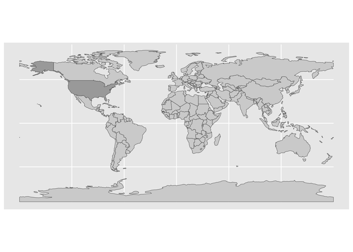
eez_gpkg <-glue("{dir_data}/raw/marineregions.org/World_EEZ_v11_20191118_gpkg/eez_v11.gpkg")# land ----ply_land_notusa <-ne_countries(scale="small", returnclass="sf") |>filter(name !="United States of America")ply_usa_land <-ne_countries(scale ="small", returnclass="sf",country ="United States of America")# plot(ply_land["name"])# mapView(ply_usa_land, zcol = "name")ggplot() +geom_sf(data = ply_land_notusa, fill ="lightgray") +geom_sf(data = ply_usa_land, fill ="darkgray")
# ply_usa$TERRITORY1 |> sort() |> paste(collapse = '", "') |> cat()# select states, ie non-territorial recognized USAply_usa <- ply_usa_terr |>filter( territory1 %in%c("Alaska", "Hawaii", "United States"), pol_type =="200NM") # exclude:# - "Overlapping claim: Puerto Rico / Dominican Republic"# - "Joint regime area United States / Russia"# simplify for plottingply_usa_s05 <- ply_usa |>ms_simplify(keep=0.05, keep_shapes=T) |>st_shift_longitude()mapView( ply_usa_s05,zcol ="territory1",layer.name ="usa.territory1<br><small>(simplified to 5%)</small>")
Source Code
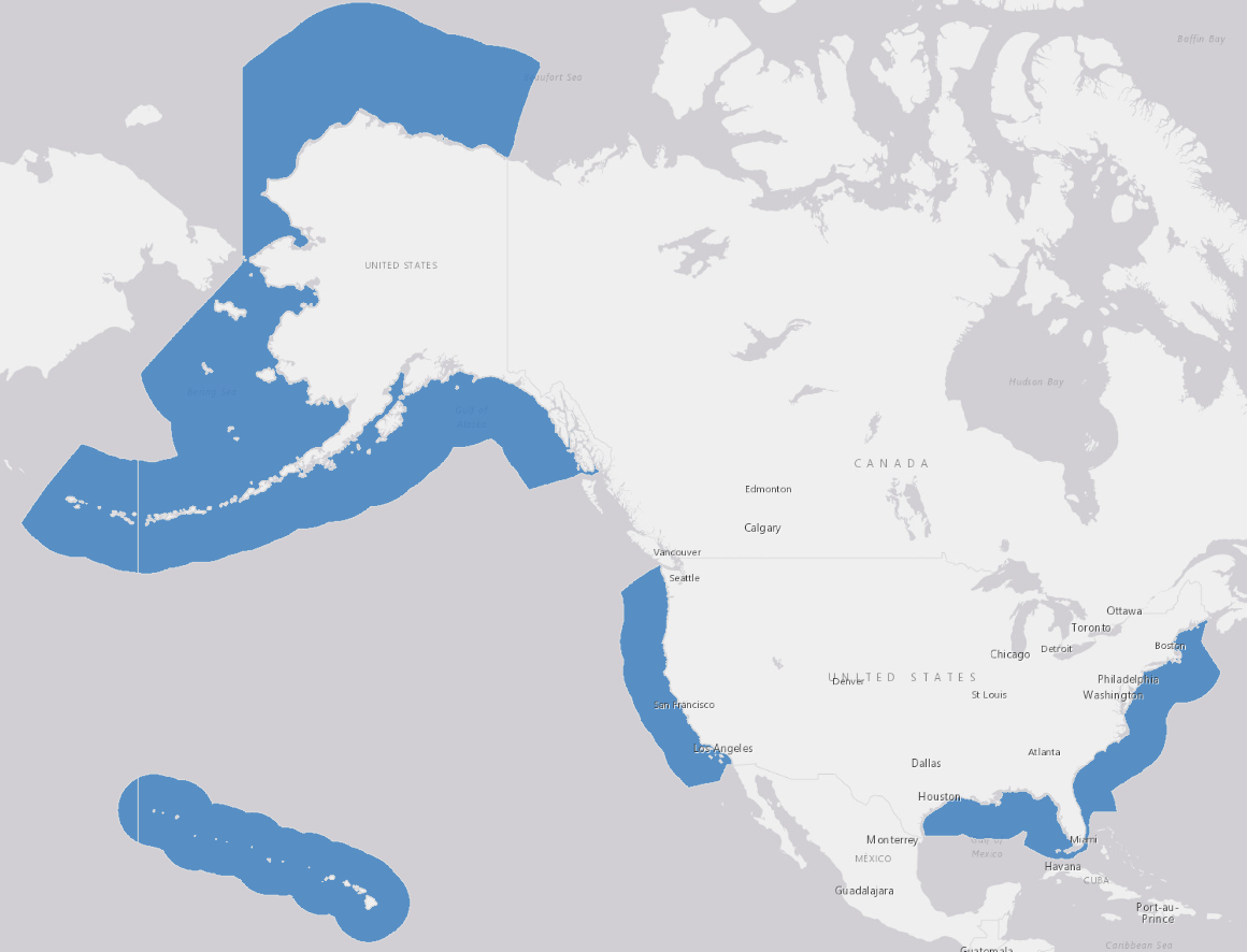
---title: "explore_regions"default-image-extension: ""---## Overview {.unnumbered}### Issues {.unnumbered}- [**objectives**#1: setup US BOEM regions for oil & gas, offshore wind](https://github.com/MarineSensitivities/objectives/issues/1) - [**workflows**#1: describe spatial units across US BOEM regions for oil & gas, offshore wind](https://github.com/MarineSensitivities/workflows/issues/1) - [**msens**#1: load BOEM spatial units into R package as locally available dataset where not too big](https://github.com/MarineSensitivities/msens/issues/1)## `ms_rgns`: BOEM Planning Areas x Outer Continental Shelf Lands Act- [BOEM Offshore Oil and Gas Planning Areas \| ArcGIS Online](https://www.arcgis.com/home/item.html?id=576ae15675d747baaec607594fed086e)\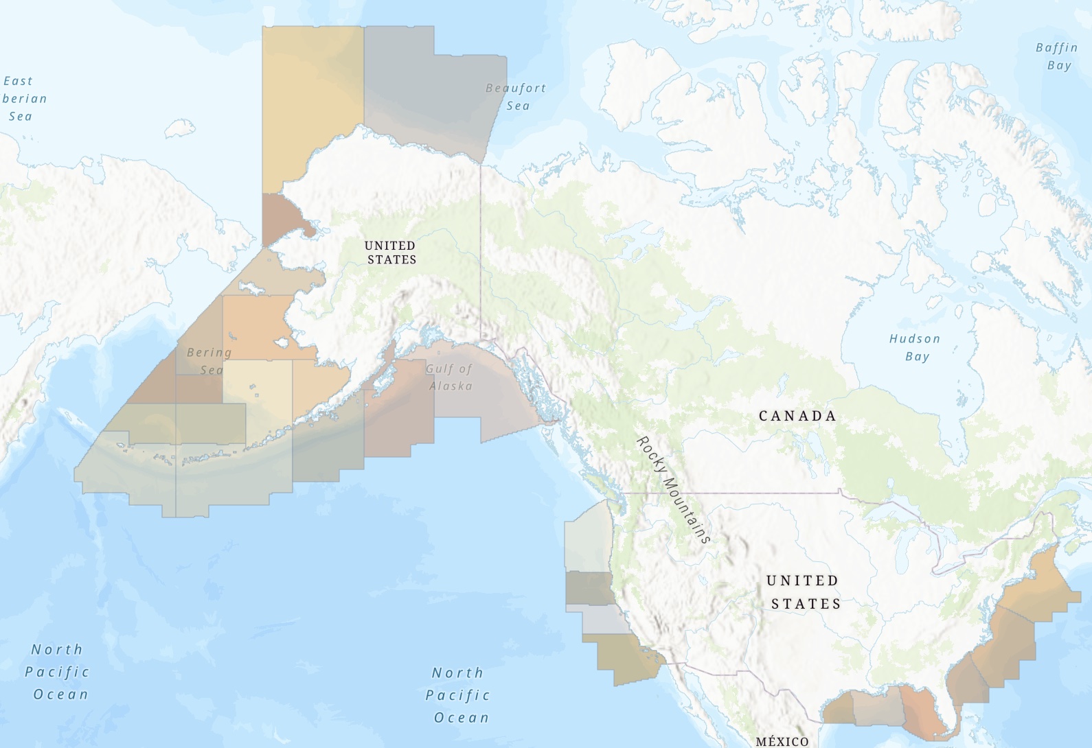\ Note: Does not include Hawaii and extends beyond EEZ.- [Outer Continental Shelf Lands Act \| MarineCadastre](https://marinecadastre-noaa.hub.arcgis.com/datasets/noaa::outer-continental-shelf-lands-act/about)```{r ms_rgns}# libraries ----librarian::shelf( dplyr, glue, janitor, here, knitr, mapview, rmapshaper, sf)# paths ----dir_data <-"/Users/bbest/My Drive/projects/msens/data"shelf_geo <-glue("{dir_data}/raw/marinecadastre.gov/Outer_Continental_Shelf_Lands_Act.geojson")plan_gdb <-glue("{dir_data}/raw/marinecadastre.gov/OffshoreOilGasPlanningArea/OilandGasPlanningAreas.gdb")rgns_geo <-here("data/ms_rgns.geojson")rgns_s05_geo <-here("data/ms_rgns_s05.geojson")shlfs_geo <-here("data/ms_shlfs.geojson")shlfs_s05_geo <-here("data/ms_shlfs_s05.geojson")# shelf ----ply_shelf <-read_sf(shelf_geo) |>st_transform(4326) |>select(objectid) |>mutate(# fix weird standalone sliver around Prince Rupertobjectid =case_match( objectid, 5~7,.default = objectid)) |>group_by(objectid) |>summarize(.groups ="drop")ply_shelf |>ms_simplify(keep=0.05, keep_shapes=T) |>st_shift_longitude() |>mapView(zcol ="objectid", layer.name ="shelf.objectid")# plan ----# st_layers(plan_gdb) # OilandGasPlanningAreasply_plan <-read_sf(plan_gdb) |>clean_names() |>select(mms_plan_a, region) |>st_transform(4326)ply_plan |>ms_simplify(keep=0.05, keep_shapes=T) |>mapView(zcol ="region", layer.name ="plan.region")# plan X shelf ----suppressWarnings({ ply_rgns <-st_intersection(ply_shelf, ply_plan) |>st_make_valid() |>group_by(objectid, mms_plan_a, region) |>summarize(.groups ="drop") |>rbind( ply_shelf |>filter(objectid %in%c(1,2)) |>mutate(mms_plan_a ="HI",region ="Hawaii")) |>st_shift_longitude()})# flag repeats from being on either side of antimeridiand_m <- ply_rgns |>st_drop_geometry() |>group_by(mms_plan_a) |>mutate(n =n()) |>filter(n >1) |>mutate(antimeridian_bearing =case_match( objectid,1~"West",2~"East",6~"West",7~"East"))|>select(-n) |>arrange(mms_plan_a, antimeridian_bearing)kable(d_m)ply_rgns <- ply_rgns |>left_join( d_m |>select(objectid, mms_plan_a, antimeridian_bearing),by =c("objectid","mms_plan_a")) |>select(-objectid) |>arrange(mms_plan_a, antimeridian_bearing) |>mutate(ctr =st_centroid(geometry),ctr_lon = ctr |>st_coordinates() %>% .[,"X"],ctr_lat = ctr |>st_coordinates() %>% .[,"Y"]) |>select(-ctr) |>mutate(shlf_name =case_when( ctr_lat <45& ctr_lon <-120& ctr_lon >-130~"Pacific", ctr_lon >-100& ctr_lon <-82~"Gulf of Mexico", ctr_lon >-82& ctr_lon <70~"Atlantic", mms_plan_a =="HI"~"Hawaii",.default ="Alaska"),shlf_key =case_match( shlf_name,"Pacific"~"PAC","Gulf of Mexico"~"GOM","Atlantic"~"ATL","Hawaii"~"HI","Alaska"~"AK")) |>rename(rgn_key = mms_plan_a,rgn_name = region)# show rgns with antimeridian_bearingply_rgns |>filter(!is.na(antimeridian_bearing)) |>ms_simplify(keep=0.05, keep_shapes=T) |>mapView(zcol ="antimeridian_bearing",layer.name ="ply_rgns.antimeridian_bearing")ply_shlfs <- ply_rgns |>group_by(shlf_key, shlf_name) |>summarize(.groups="drop") |>mutate(ctr =st_centroid(geometry),ctr_lon = ctr |>st_coordinates() %>% .[,"X"],ctr_lat = ctr |>st_coordinates() %>% .[,"Y"]) |>select(-ctr) |>st_shift_longitude() |>mutate(area_km2 =st_area(geometry) |> units::set_units(km^2) |>as.numeric()) |>relocate(geometry, .after =last_col()) |>arrange(shlf_name)# writewrite_sf(ply_shlfs, shlfs_geo, delete_dsn=T)# simplifyply_shlfs_s05 <- ply_shlfs |>ms_simplify(keep=0.05, keep_shapes=T)write_sf(ply_shlfs_s05, shlfs_s05_geo, delete_dsn=T)# ply_rgns dissolved to rgnply_rgns <- ply_rgns |>group_by(shlf_key, shlf_name, rgn_key, rgn_name) |>summarize(.groups="drop") |>mutate(ctr =st_centroid(geometry),ctr_lon = ctr |>st_coordinates() %>% .[,"X"],ctr_lat = ctr |>st_coordinates() %>% .[,"Y"]) |>select(-ctr) |>st_shift_longitude() |>mutate(area_km2 =st_area(geometry) |> units::set_units(km^2) |>as.numeric()) |>arrange(shlf_name, rgn_name) |>relocate(geometry, .after =last_col())# write write_sf(ply_rgns, rgns_geo, delete_dsn=T)# simplifyply_rgns_s05 <- ply_rgns |>ms_simplify(keep=0.05, keep_shapes=T)write_sf(ply_rgns_s05, rgns_s05_geo, delete_dsn=T)# read and mapply_rgns_s05 <-read_sf(rgns_s05_geo)ply_rgns <-read_sf(rgns_geo)mapView( ply_rgns_s05 |>mutate(shlf_rgn_name =glue("{shlf_name} - {rgn_name}"),shlf_rgn_key =glue("{shlf_key} - {rgn_key}")),zcol ="shlf_rgn_key",layer.name ="shlf_rgn_key<br><small>(simplified to 5%)</small>")```### TODO (issues to add):- Fix weird pixelation in Alaska: Aleutian Arc, Shumagin, St. Matthew-Hall## Questions1. Are the above sites contain the authoritative sources or should we pull from elsewhere? > Other tools such as [OceanReports](https://marinecadastre.gov/oceanreports) and the Environmental Studies Program Information System - [ESPIS](https://esp-boem.hub.arcgis.com/) can also be found from the [MarineCadastre.gov](https://marinecadastre.gov/) site.2. Also include [**OPD, SOBD, CBD, & Lease Map Diagrams**](https://www.boem.gov/oil-gas-energy/mapping-and-data#:~:text=OPD%2C%20SOBD%2C%20CBD%2C%20%26%20Lease%20Map%20Diagrams)? > Official Protraction Diagrams (OPDs) and Lease Maps show the OCS block grids and other boundaries for a given area. Supplemental Official Block Diagrams (SOBDs) are created for individual blocks which are intersected by offshore boundaries. The zip files may contain both current and historic SOBDs. The older SOBDs are provided for historical reference, but all future activities will be based on the most current SOBDs. Composite Block Diagrams (CBDs) show NAD 27 lease information portrayed on the NAD 83 cadastre, or show other boundaries that have changed over time. Not all OPDs have SOBDs or CBDs associated with them.## OLD### EEZThe Exclusive Economic Zone determines US jurisdiction. Federal jurisdiction does not apply until 12 nm offshore though where it is state jurisdiction.Presumably we are only interested in the U.S. non-territorial waters, i.e. that of the states...```{r eez}librarian::shelf( DT, ggplot2, rnaturalearth, rnaturalearthdata, ropensci/rnaturalearthhires, stringr, units)eez_gpkg <-glue("{dir_data}/raw/marineregions.org/World_EEZ_v11_20191118_gpkg/eez_v11.gpkg")# land ----ply_land_notusa <-ne_countries(scale="small", returnclass="sf") |>filter(name !="United States of America")ply_usa_land <-ne_countries(scale ="small", returnclass="sf",country ="United States of America")# plot(ply_land["name"])# mapView(ply_usa_land, zcol = "name")ggplot() +geom_sf(data = ply_land_notusa, fill ="lightgray") +geom_sf(data = ply_usa_land, fill ="darkgray")# eez ----# st_layers(eez_gpkg, do_count = T) # eez_v11ply_eez <-st_read(eez_gpkg)# mapView(ply_eez) # too big# idx_valid <- st_is_valid(ply_eez)# ply_eez |> # filter(!idx_valid) |> # st_drop_geometry() |> # pull(GEONAME) # "Canadian Exclusive Economic Zone" "Russian Exclusive economic Zone" ply_usa_terr <- ply_eez |>clean_names() |># make fields lowercasefilter( sovereign1 =="United States") |>select(mrgid, territory1, pol_type, geoname, area_km2) |>arrange(territory1) |>st_shift_longitude()# simplify for plottingply_usa_terr_s05 <- ply_usa_terr |>ms_simplify(keep=0.05, keep_shapes=T)mapView( ply_usa_terr_s05,zcol ="territory1",layer.name ="usa_terr.territory1<br><small>(simplified to 5%)</small>")ply_usa_terr_s05 |>st_drop_geometry() |>relocate(mrgid, .after = geoname) |>datatable(options =list(paging=F, dom="t")) |>formatRound("area_km2", digits =0, mark =",")# ply_usa$TERRITORY1 |> sort() |> paste(collapse = '", "') |> cat()# select states, ie non-territorial recognized USAply_usa <- ply_usa_terr |>filter( territory1 %in%c("Alaska", "Hawaii", "United States"), pol_type =="200NM") # exclude:# - "Overlapping claim: Puerto Rico / Dominican Republic"# - "Joint regime area United States / Russia"# simplify for plottingply_usa_s05 <- ply_usa |>ms_simplify(keep=0.05, keep_shapes=T) |>st_shift_longitude()mapView( ply_usa_s05,zcol ="territory1",layer.name ="usa.territory1<br><small>(simplified to 5%)</small>")```