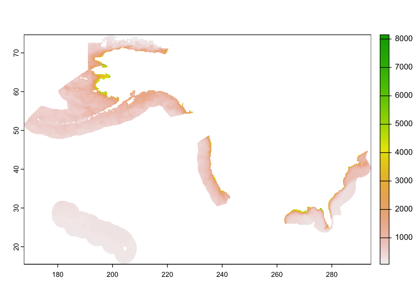
Community guidance for developing this website was to provide a single productivity product as a Standard product. For this, we initially chose the original Vertically Generalized Production Model (VGPM) (Behrenfeld and Falkowski, 1997a) as the standard algorithm. The VGPM is a “chlorophyll-based” model that estimate net primary production from chlorophyll using a temperature-dependent description of chlorophyll-specific photosynthetic efficiency. For the VGPM, net primary production is a function of chlorophyll, available light, and the photosynthetic efficiency. Shown below is an example of VGPM-based global ocean net primary production for July of 2016.
Standard products are based on chlorophyll, temperature and PAR data from SeaWiFS, MODIS and VIIRS satellites, along with estimates of euphotic zone depth from a model developed by Morel and Berthon (1989) and based on chlorophyll concentration. Monthly global ocean production for July 2016 was 4.43626 Pg (1 Pg = 10**15 g.)
vgpm.m.2021.tar (48 MB) downloaded into dir_vgpm from:
---title: "explore_productivity"editor_options: chunk_output_type: console---Primary Productivity from:- [Ocean Productivity | Oregeon State](http://sites.science.oregonstate.edu/ocean.productivity/)- Calculated mean from 2021 monthlies> Community guidance for developing this website was to provide a singleproductivity product as a Standard product. For this, we initially chose the original Vertically Generalized Production Model (VGPM) (Behrenfeld and Falkowski, 1997a) as the standard algorithm. The VGPM is a "chlorophyll-based" model that estimate net primary production from chlorophyll using a temperature-dependent description of chlorophyll-specific photosynthetic efficiency. For the VGPM, net primary production is a function of chlorophyll, available light, and the photosynthetic efficiency. Shown below is an example of VGPM-based global ocean net primary production for July of 2016.>> Standard products are based on chlorophyll, temperature and PAR data from SeaWiFS, MODIS and VIIRS satellites, along with estimates of euphotic zone depth from a model developed by Morel and Berthon (1989) and based onchlorophyll concentration. Monthly global ocean production for July 2016 was 4.43626 Pg (1 Pg = 10**15 g.)vgpm.m.2021.tar (48 MB) downloaded into dir_vgpm from:* [Ocean Productivity: Online VGPM Data](http://orca.science.oregonstate.edu/1080.by.2160.monthly.hdf.vgpm.m.chl.m.sst.php)See [Ocean Productivity: Frequently AskedQuestions](http://orca.science.oregonstate.edu/faq01.php)### CitationFor citation, please reference the original vgpm paper by [Behrenfeld and Falkowski, 1997a](http://science.oregonstate.edu/ocean.productivity/references.php#Behrenfeld.1997a)as well as the [Ocean Productivity](http://science.oregonstate.edu/ocean.productivity/index.php) site for the data.```{r}librarian::shelf( DBI, devtools, dplyr, exactextractr, fs, glue, leaflet, purrr, R.utils, sf, terra,quiet = T)devtools::load_all("~/Github/MarineSensitivities/msens")dir_data <-"/Users/bbest/My Drive/projects/msens/data"dir_vgpm <-glue("{dir_data}/raw/oregonstate.edu/vgpm.m.2021")hdf2nc <-glue("{dir_data}/raw/oregonstate.edu/software/h4tonccf_nc4")vgpm_tif <-glue("{dir_data}/derived/vgpm_2021.tif")stopifnot(all(dir_exists(dir_data),dir_exists(dir_vgpm),file_exists(hdf2nc),dir_exists(dirname(vgpm_tif)) ) )if (!file_exists(vgpm_tif)){# unzip from *.gz to *.hdf ---- gzs <-list.files(dir_vgpm, "\\.gz$", full.names=T)lapply(gzs, gunzip)# convert from *.hdf to *.nc ----# download [h4tonccf_nc4](https://www.hdfeos.org/software/h4cflib.php)# and add to directory; chmod o+x h4tonccf_nc4; allow to run in OS Settings hdfs <-list.files(dir_vgpm, ".hdf", full.names=T) ncs <-path_ext_set(hdfs, "nc") idx_nc <-!file.exists(ncs) cmds <-glue("cd '{dir_vgpm}'; '{hdf2nc}' {basename(hdfs[idx_nc])}")sapply(cmds, system)sapply(hdfs, file_delete)# convert nc to tif, projected and clipped to OffHab raster ----# * get bounding box for clipping global raster ---- bb <- msens::ply_shlfs |>st_bbox() r_cid <-oh_rast("cell_id") bb_oh_b1dd_gcs <- r_cid %>%ext() %>%st_bbox() %>%st_as_sfc() %>%st_as_sf() %>%st_set_crs(3857) %>%st_transform(4326) %>%st_set_crs(NA) %>%st_buffer(1) %>%st_set_crs(4326)# mapview::mapView(bb_oh_b1dd_gcs) nc_to_oh_tif <-function(nc, i=0){# nc = ncs[1]; i=0 tif <-glue("{path_ext_remove(nc)}_ms.tif")message(glue("{i}: {basename(nc)} -> {basename(tif)}"))# read netcdf as raster# set extent and coordinate reference system and NA r <-rast(nc) |>flip(direction="vertical")ext(r) <-c(-180, 180, -90, 90)crs(r) <-"EPSG:4326" r <-rotate(r, left=F) r[r==-9999] <-NA# plot(r) r <- r |>crop(bb) |>mask(vect(msens::ply_shlfs))# plot(r)writeRaster(r, tif, overwrite=T) }list.files(dir_vgpm, "\\.nc$", full.names=T) |>iwalk(nc_to_oh_tif)}# calculate annual mean from monthly tifs ----tifs <-list.files(dir_vgpm, "\\.tif$", full.names=T)r_ms <-rast(tifs)r <-mean(r_ms, na.rm=T)plot(r)writeRaster(r, vgpm_tif, overwrite=T)base_opacity <-0.7m <-leaflet() |># add base: blue bathymetry and light brown/green topography leaflet::addProviderTiles("Esri.OceanBasemap",options =providerTileOptions(variant ="Ocean/World_Ocean_Base",opacity = base_opacity)) |># add reference: placename labels and borders leaflet::addProviderTiles("Esri.OceanBasemap",options =providerTileOptions(variant ="Ocean/World_Ocean_Reference",opacity = base_opacity))# east of antimeridianr_e <-shift(r, -360) |>crop(ext(-180,180,-90,90), snap="in")# plot(r_e)# west of antimeridianr_w <- r |>crop(ext(-180,180,-90,90), snap="in")# plot(r_w)pal <-colorNumeric("Spectral", na.color ="transparent",domain =range(values(r, na.rm=T)))m |>addRasterImage(r_e, colors = pal, opacity=0.8) |>addRasterImage(r_w, colors = pal, opacity=0.8) |>addLegend(pal = pal, values =values(r, na.rm=T),title ="Productivity<br><small>(mg C/m<sup>2</sup>/day)<small>")global(r, "mean", na.rm=T)# mean cell value, weighted by the fraction of each cell that is covered by the polygonp <- msens::ply_rgns_s05 |>mutate(vgpm =exact_extract(r, msens::ply_rgns, "mean", progress=F))pal <-colorNumeric("Spectral", na.color ="transparent",domain = p$vgpm)m |>addPolygons(data = p,fillColor =~pal(vgpm),fillOpacity =0.7,color ="gray",weight =1,opacity =0.8,highlightOptions =highlightOptions(weight =2,color ="black",fillOpacity =0.8,opacity =0.9,bringToFront = T)) |>addLegend(data = p,pal = pal, values =~vgpm, opacity =0.8, title ="Productivity<br><small>(mg C/m<sup>2</sup>/day)<small>",position ="bottomright")# s <- p |> # group_by(# shlf_key, shlf_name) |># summarize(# vgpm = weighted.mean(vgpm, area_km2, na.rm=T))s <- msens::ply_shlfs_s05 |>mutate(vgpm =exact_extract(r, msens::ply_shlfs, "mean", progress=F))pal <-colorNumeric("Spectral", na.color ="transparent",domain = s$vgpm)m |>addPolygons(data = s,fillColor =~pal(vgpm),fillOpacity =0.7,color ="gray",weight =1,opacity =0.8,highlightOptions =highlightOptions(weight =2,color ="black",fillOpacity =0.8,opacity =0.9,bringToFront = T)) |>addLegend(data = s,pal = pal, values =~vgpm, opacity =0.8, title ="Productivity<br><small>(mg C/m<sup>2</sup>/day)<small>",position ="bottomright")```