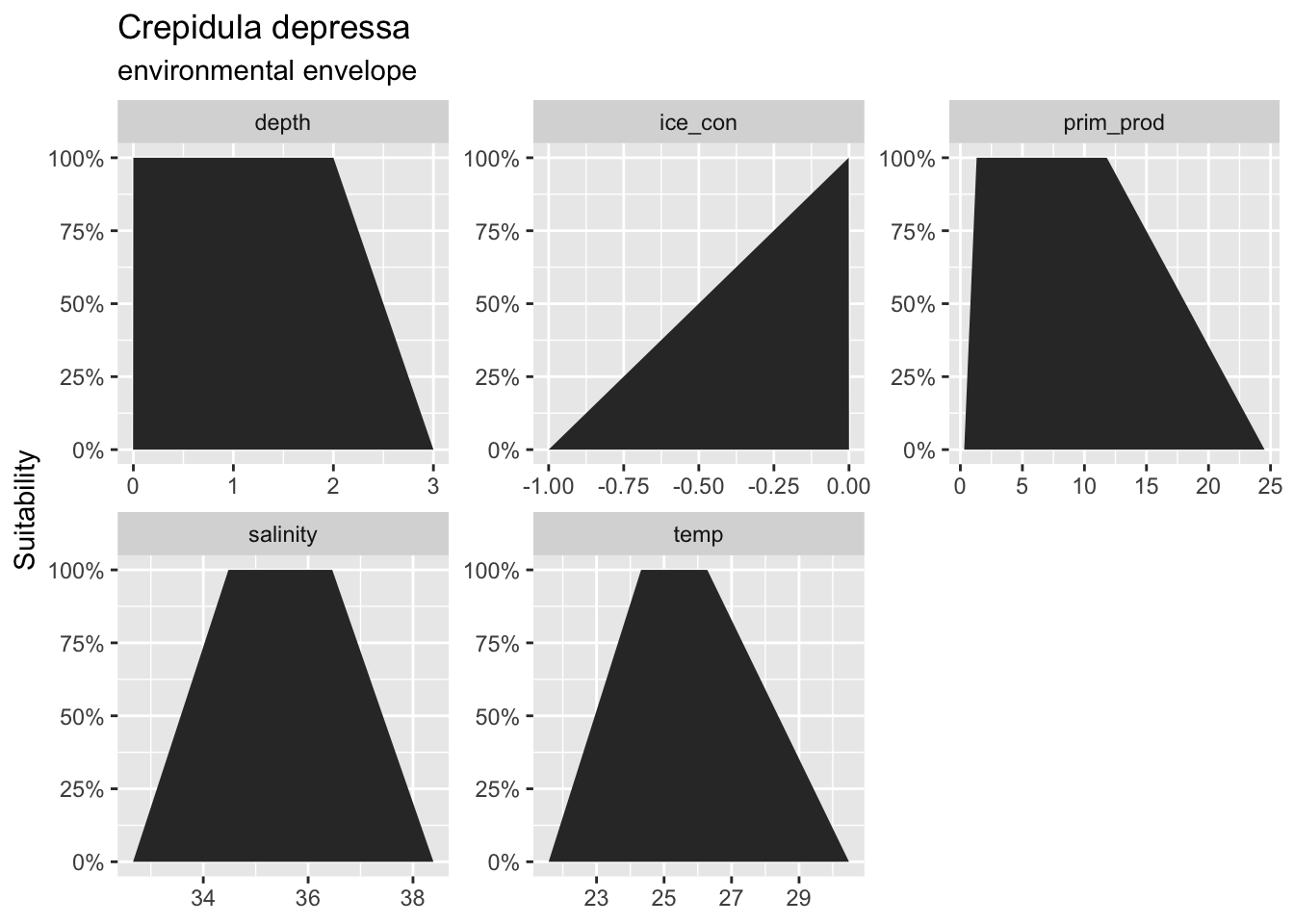
Explore Interpolation of SDMs

Sources:

• AquaMaps raster from env REsuitability
  • Get a few species with different geographic traits, starting with species in Gulf of America:
    • small range, high density
    • large range, low density
• Bottom Trawl from IDW
• Other: GoMex hexagons from complex SDM

Topologies:

• raster:
  • 1/12° (0.083°)
    CopernicusMarine VGPM
  • 1/20° (0.050°)
    BioOracle
• hexagon:
  • Uber H3

Methods:

• “chunky”: interpolate from underlying values
• “smooth”: interpolate from centroid points
• “remap”: re-ramp environmental envelope from higher resolution data
  • only AquaMaps, possibly DisMAP

Background:

• MarineSDMs - Explorations
• MarineSDMs - AquaMaps Downscaled
• marinebon/aquamaps-downscaled: initial attempt to downscale AquaMaps species distribution models to finer spatial resolution a la GEBCO bathymetry (15 arc second)
• aquamaps-downscaled/index.qmd at main · marinebon/aquamaps-downscaled
• Downscaling AquaMaps
• aquamaps-downscaled/am-env_to_ee.qmd at main · marinebon/aquamaps-downscaled

1 AquaMaps duckdb database

librarian::shelf(
  cmocean, DBI, dplyr, DT, duckdb, fs, glue, here, htmltools, janitor, knitr,
  leaflet, leaflet.extras, librarian, mapview,
  # raquamaps/raquamaps,
  marinesensitivity/msens,
  RColorBrewer, readr, sf, stringr, terra, tibble, tidyr,
  quiet = T)  # zeallot
mapviewOptions(basemaps = "Esri.OceanBasemap")

dir_data <- "~/My Drive/projects/msens/data"
path_dd  <- glue("{dir_data}/derived/aquamaps/am.duckdb")

con_dd   <- dbConnect(
  duckdb(
    dbdir     = path_dd,
    read_only = T))
# dbDisconnect(con_dd, shutdown = T)
# dbListTables(con_dd)
#   "_tbl_fld_renames" "cells" "spp" "spp_cells" "spp_occs" "spp_prefs"
tbl(con_dd, "_tbl_fld_renames") |> 
  collect() |> 
  datatable()

2 Gulf of America

R package msens: ply_boemrgns > ply_ecorgns | ply_planareas > ply_ecoareas

TODO:

• Rename Gulf of Mexico to Gulf of America
  • boemrgn_key: “brGOM” -> “brGOA”
  • boemrgn_name: “Gulf of Mexico” -> “Gulf of America”

# st_bbox(msens::ply_boemrgns)
#      xmin      ymin      xmax      ymax 
# 166.95776  23.78077 295.89167  74.99636
#   so [0,360], not [-180, 180]

goa <- msens::ply_boemrgns |> 
  filter(boemrgn_key == "brGOM") |> 
  st_wrap_dateline()    # [   0, 360] -> [-180, 180]
# st_shift_longitude()  # [-180, 180] -> [    0,360]

# st_bbox(goa)
# xmin      ymin      xmax      ymax 
# -97.23899  23.78077 -81.17011  30.28910
mapView(goa)

3 Get species in Gulf of America

# get cells within goa
pt_cell <- tbl(con_dd, "cells") |> 
  collect() |> 
  st_as_sf(
    coords = c("center_long", "center_lat"), crs = 4326, remove = F)
pt_cell_goa <- st_intersection(pt_cell, goa)

# get species in gom
d_sp_goa <- tbl(con_dd, "spp_cells") |> 
  filter(cell_id %in% pt_cell_goa$cell_id) |>
  group_by(sp_key) |>
  collect()

# get species ranges by n_cells
d_sp_goa_rng <- tbl(con_dd, "spp_cells") |> 
  filter(sp_key %in% d_sp_goa$sp_key) |> 
  group_by(sp_key) |>
  summarize(
    n_cells = n(), .groups = "drop") |>
  left_join(
    tbl(con_dd, "spp"), 
    by = "sp_key") |>
  arrange(n_cells) |> 
  collect()

bind_rows(
  slice(d_sp_goa_rng, 1:100),
  slice(d_sp_goa_rng, (n() - 99):n())) |> 
  datatable(
    caption = htmltools::tags$caption(
      style = 'caption-side: top; text-align: left;',
      withTags(div(HTML(
        glue("
      Table. <i>Species in Gulf of America (n = {format(nrow(d_sp_goa_rng), big.mark=',')}), 
      subset to first 100 species and last 100 species,
      sorted by range size (n_cells).</i>"))))))

4 Get AquaMaps env data

# source: https://github.com/marinebon/aquamaps-downscaled/blob/main/am-env_to_ee.qmd

h_tif  <- here("data/am-hcaf.tif")

if (!file.exists(h_tif)){
  # get aquamaps table of env values ----
  # d_cells <- tbl(con_dd, "cells") |> 
  #   collect()
  
  # raster template ----
  # range(d$ctr_lon)  # -179.75  179.75
  # range(d$ctr_lat)  # - 78.25   89.75
  # r_template <- rast(
  #   xmin       = min(d_cells$center_long) - 0.25,
  #   xmax       = max(d_cells$center_long) + 0.25,
  #   ymin       = min(d_cells$center_lat) - 0.25,
  #   ymax       = max(d_cells$center_lat) + 0.25,
  #   resolution = c(0.5, 0.5),
  #   crs = "epsg:4326")
  
  # Create the global template raster
  xmin <- -180; xmax <- 180
  ymin <-  -90; ymax <-  90
  res  <-    0.5  # Half-degree resolution
  
  r_g <- rast(
    nrows = (ymax - ymin) / res,
    ncols = (xmax - xmin) / res,
    xmin = xmin,
    xmax = xmax,
    ymin = ymin,
    ymax = ymax,
    crs = "EPSG:4326")
  
  # data frame to points ----
  p <- tbl(con_dd, "cells") |> 
    collect() |>
    st_as_sf(
      coords = c("center_long", "center_lat"),
      remove = F,
      crs    = 4326) |> 
    arrange(center_long, center_lat)

  # points to raster ----
  get_r <- function(v){
    r <- rasterize(p, r_g, field = v)
    names(r) <- v
    r
  }
  
  r_h <- NULL
  for (v in setdiff(names(p), "geometry")){
    message(glue("v: {v}"))
    
    if (is.null(r_h)){
      r_h <- get_r(v)
    } else {
      r_h <- rast(list(r_h, get_r(v)))
    }
  }
  
  writeRaster(r_h, h_tif, overwrite=T)
}
r_h <- rast(h_tif)

# names(r_h)
#  [1] "cell_id"            "cell_idx"           "csquare_code"       "loiczid"           
#  [5] "n_limit"            "s_limit"            "w_limit"            "e_limit"           
#  [9] "center_lat"         "center_long"        "cell_area"          "ocean_area"        
# [13] "p_water"            "clim_zone_code"     "fao_area_m"         "fao_area_in"       
# [17] "country_main"       "country_second"     "country_third"      "country_sub_main"  
# [21] "country_sub_second" "country_sub_third"  "eez"                "lme"               
# [25] "lme_border"         "meow"               "ocean_basin"        "islands_no"        
# [29] "area0_20"           "area20_40"          "area40_60"          "area60_80"         
# [33] "area80_100"         "area_below100"      "elevation_min"      "elevation_max"     
# [37] "elevation_mean"     "elevation_sd"       "depth_min"          "depth_max"         
# [41] "depth_mean"         "depth_sd"           "sst_an_mean"        "sbt_an_mean"       
# [45] "salinity_mean"      "salinity_b_mean"    "prim_prod_mean"     "ice_con_ann"       
# [49] "oxy_mean"           "oxy_b_mean"         "land_dist"          "shelf"             
# [53] "slope"              "abyssal"            "tidal_range"        "coral"             
# [57] "estuary"            "seamount"           "mpa"

# plot to check
#  static:
#    plot(r_h[["center_lat"]])
#    plot(r_h[["center_long"]])
#  dynamic:
#    plet(r_h[["center_lat"]])
#    plet(r_h[["center_long"]])

lyr <- "depth_mean"; clr <- "dense"
mapView(
  r_h[[lyr]], layer.name = lyr,
  col.regions = cmocean(clr),
  alpha.regions = 0.9)

lyr <- "prim_prod_mean"; clr <- "algae"
mapView(
  r_h[[lyr]], layer.name = lyr,
  col.regions = cmocean(clr),
  alpha.regions = 0.9)

lyr <- "sst_an_mean"; clr <- "thermal"
mapView(
  r_h[[lyr]], layer.name = lyr,
  col.regions = cmocean(clr),
  alpha.regions = 0.9)

lyr <- "sbt_an_mean"; clr <- "thermal"
mapView(
  r_h[[lyr]], layer.name = lyr,
  col.regions = cmocean(clr),
  alpha.regions = 0.9)

5 Get species attributes

• Computer Generated Native Distribution Map for Crepidula depressa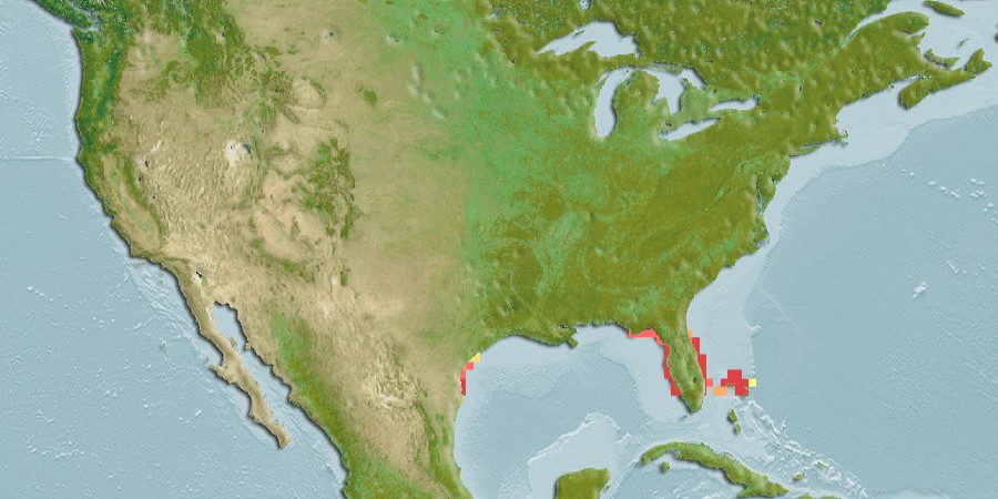

• Mapping Parameters

• "W-Msc-419703": Crepidula depressa (class = Gastropoda) n_cells = 50

sp_key <- "W-Msc-419703"

d_sp_pref <- tbl(con_dd, "spp_prefs") |> 
  filter(sp_key == !!sp_key) |> 
  collect()

d_sp_pref |> 
  mutate(across(everything(), as.character)) |> 
  pivot_longer(everything()) |> 
  kable()

name	value
sp_key	W-Msc-419703
sp_int	151110
life_stage	adults
fao_areas	31
fao_complete	NA
n_most_lat	30
s_most_lat	26
w_most_long	97
e_most_long	80
depth_yn	1
depth_min	0
depth_pref_min	0
depth_pref_max	2
depth_max	3
mean_depth	NA
pelagic	0
temp_yn	1
temp_min	21.58
temp_pref_min	24.32
temp_pref_max	26.28
temp_max	30.48
salinity_yn	1
salinity_min	32.66
salinity_pref_min	34.48
salinity_pref_max	36.46
salinity_max	38.39
prim_prod_yn	1
prim_prod_min	0.31
prim_prod_pref_min	1.31
prim_prod_pref_max	11.8
prim_prod_max	24.52
ice_con_yn	1
ice_con_min	-1
ice_con_pref_min	0
ice_con_pref_max	0
ice_con_max	0
oxy_yn	0
oxy_min	194.25
oxy_pref_min	205.66
oxy_pref_max	215.66
oxy_max	227.88
land_dist_yn	0
land_dist_min	7
land_dist_pref_min	10
land_dist_pref_max	24
land_dist_max	75
remark	NA
date_created	2019-08-07 00:00:00
date_modified	NA
expert_id	NA
date_expert	NA
layer	s
rank	1
map_opt	1
extn_rule_yn	1
reviewed	NA

TODO:

• Reconcile differences in bbox and FAO areas vs online.

librarian::shelf(
  ggplot2, listviewer, scales)

get_sp_info <- function(sp_key){
# source: https://github.com/marinebon/aquamaps-downscaled/blob/503c62f39552c4ad2417413b13c49d4d4405f3ab/sp-map/functions.R#L92C5-L93C30

  d_prefs <- tbl(con_dd, "spp_prefs") |> 
      filter(sp_key == !!sp_key) |>
      collect()

  vars_yes <- d_prefs |> 
    select(ends_with("_yn")) |> 
    pivot_longer(
      everything()) |> 
    filter(value == 1) |> 
    pull(name) |> 
    str_replace("_yn$","") |> 
    setdiff("extn_rule")
  
  d_probs <- tribble(
    ~prob_name, ~prob_value,
    "min"     , 0,
    "pref_min", 1,
    "pref_max", 1,
    "max"     , 0)
  
  # browser()
  d_env <- d_prefs |> 
    select(starts_with(vars_yes)) |>
    select(!ends_with("_yn")) |> 
    pivot_longer(
      everything(),
      values_to = "var_value") |> 
    separate_wider_regex(
      name,
      c(var       = paste(vars_yes, collapse = "|"),
        "_",
        prob_name = paste(d_probs$prob_name, collapse = "|"))) |> 
    left_join(
      d_probs,
      by = "prob_name")
  
  l_env <- d_env |> 
    group_by(var) |> 
    summarise(
      vec = list(var_value)) |> 
    deframe()
  
  sp_info <- list()
  
  d_sp <- tbl(con_dd, "spp") |> 
    filter(sp_key == !!sp_key) |> 
    collect() |> 
    mutate(
      sp_sci = glue("{genus} {species}"))
  sp_info["sp_scientific"] <- list(d_sp$sp_sci)
  sp_info["sp_key"]        <- list(d_sp$sp_key)
  sp_info["sp_int"]        <- list(d_sp$sp_int)
  
  sp_info["fao_areas"] <- d_prefs$fao_areas |> 
    str_split(",\\s*") |> 
    str_trim() |> 
    unlist() |> 
    as.numeric() |> 
    sort()
  
  sp_info["env"] <- list(l_env)
  
  sp_info$taxa <- d_sp |> 
      select(kingdom, phylum, class, order, family) |> 
      pivot_longer(everything()) |> 
      deframe() |> 
      as.list()
  
  sp_info$attr <- d_sp |> 
    select(
      deepwater, angling, diving, dangerous, m_invertebrates, 
      highseas, invasive, resilience) |> 
    mutate(across(everything(), as.character)) |> 
    pivot_longer(everything()) |> 
    deframe() |> 
    as.list()
  
  sp_info$iucn <- d_sp |> 
    select(
      iucn_id, iucn_code, iucn_version, provider) |> 
    mutate(across(everything(), as.character)) |> 
    pivot_longer(everything()) |> 
    deframe() |> 
    as.list()
  
  # deepwater,        # Does the species occur in the deep-sea (i.e. tagged bathypelagic or bathydemersal in FishBase or SeaLifeBase)? 0=No, 1=Yes
  # angling,          # Is the species a sport fish (i.e. tagged as a GameFish in FishBase)? 0=No, 1=Yes
  # diving,           # Is the species found on a dive (i.e. where DepthPrefMin in HSPEN < 20 meters)? 0=No, 1=Yes
  # dangerous,        # Is the species dangerous (i.e. tagged as ‘traumatogenic or venonous’ in FishBase or SeaLifeBase)? 0=No, 1=Yes
  # m_invertebrates,  # Is the species a marine invertebrate? 0=No, 1=Yes
  # highseas,         # Is the species an open ocean fish species (i.e. tagged as pelagic-oceanic in FishBase)? 0=No, 1=Yes
  # invasive,         # Is the species recorded to be invasive (i.e. in FishBase or SeaLifeBase)? 0=No, 1=Yes
  # resilience,       # Resilience of the species (i.e. as recorded in FishBase/SeaLifeBase) [varchar]
  # iucn_id,          # IUCN species identifier [int]
  # iucn_code,        # IUCN Red list classification assigned to the species [varchar]
  # iucn_version,     # IUCN version [varchar]
  # provider) |>      # FishBase (FB) or SeaLifeBase (SLB)? [varchar]
  
  sp_info
}

sp_info <- get_sp_info(sp_key)

plot_sp_env <- function(sp_info){

    d <- sp_info$env |> 
      enframe(name = "variable") |> 
      mutate(
        suitability = list(c(0,1,1,0))) |> 
      unnest(c(value, suitability))
    
    g <- ggplot(d, aes(value, suitability)) +
      geom_area() +
      scale_y_continuous(labels = percent) +
      facet_wrap(
        vars(variable), 
        scales = "free") +
      labs(
        title    = sp_info$sp_scientific,
        subtitle = "environmental envelope",
        x        = NULL,
        y        = "Suitability") +
      theme_gray()
    
    g
}

plot_sp_env(sp_info)

jsonedit(
  sp_info, mode = "view", modes = c("view","code"))

6 Compare with native aquamapsdata

# dependency for aquamapsdata:
#  - Terminal: brew install gnupg
librarian::shelf(
  cran/rcrypt,
  raquamaps/aquamapsdata,
  dplyr)

# initial run-once step required to install remote db locally
# download_db(force = TRUE)

default_db("sqlite")

<SQLiteConnection>
  Path: /Users/bbest/Library/Application Support/aquamaps/am.db
  Extensions: TRUE

# get the identifier for the species
ras <- am_raster(sp_key)
b <- ext(ras) |> as.vector() |> as.numeric()

# show the native habitat map
am_map_leaflet(ras, title = sp_key) |> 
  leaflet::fitBounds(
    lng1 = b[1], lat1 = b[3], lng2 = b[2], lat2 = b[4])

#   xmin   xmax   ymin   ymax 
# -97.75 -76.75  26.25  29.75
  
# use one or more keys for species
am_hspen() |> 
  filter(SpeciesID == sp_key) |> 
  head(1) |> 
  collapse() |> 
  glimpse()

Rows: ??
Columns: 56
Database: sqlite 3.47.1 [/Users/bbest/Library/Application Support/aquamaps/am.db]
$ SpeciesID       <chr> "W-Msc-419703"
$ Speccode        <int> 151110
$ LifeStage       <chr> "adults"
$ FAOAreas        <chr> "31"
$ FAOComplete     <int> NA
$ NMostLat        <dbl> 30
$ SMostLat        <dbl> 26
$ WMostLong       <dbl> 97
$ EMostLong       <dbl> 80
$ DepthYN         <int> 1
$ DepthMin        <int> 0
$ DepthPrefMin    <int> 0
$ DepthPrefMax    <int> 2
$ DepthMax        <int> 3
$ MeanDepth       <int> NA
$ Pelagic         <int> 0
$ TempYN          <int> 1
$ TempMin         <dbl> 21.58
$ TempPrefMin     <dbl> 24.32
$ TempPrefMax     <dbl> 26.28
$ TempMax         <dbl> 30.48
$ SalinityYN      <int> 1
$ SalinityMin     <dbl> 32.66
$ SalinityPrefMin <dbl> 34.48
$ SalinityPrefMax <dbl> 36.46
$ SalinityMax     <dbl> 38.39
$ PrimProdYN      <int> 1
$ PrimProdMin     <dbl> 0.31
$ PrimProdPrefMin <dbl> 1.31
$ PrimProdPrefMax <dbl> 11.8
$ PrimProdMax     <dbl> 24.52
$ IceConYN        <int> 1
$ IceConMin       <dbl> -1
$ IceConPrefMin   <dbl> 0
$ IceConPrefMax   <dbl> 0
$ IceConMax       <dbl> 0
$ OxyYN           <int> 0
$ OxyMin          <dbl> 194.25
$ OxyPrefMin      <dbl> 205.66
$ OxyPrefMax      <dbl> 215.66
$ OxyMax          <dbl> 227.88
$ LandDistYN      <int> 0
$ LandDistMin     <dbl> 7
$ LandDistPrefMin <dbl> 10
$ LandDistPrefMax <dbl> 24
$ LandDistMax     <dbl> 75
$ Remark          <chr> NA
$ DateCreated     <chr> "2019-08-07 00:00:00"
$ DateModified    <chr> NA
$ expert_id       <int> NA
$ DateExpert      <chr> NA
$ Layer           <chr> "s"
$ Rank            <int> 1
$ MapOpt          <int> 1
$ ExtnRuleYN      <int> 1
$ Reviewed        <int> NA

# $ FAOAreas        <chr> "31"
# $ FAOComplete     <int> NA
# $ NMostLat        <dbl> 30
# $ SMostLat        <dbl> 26
# $ WMostLong       <dbl> 97
# $ EMostLong       <dbl> 80

7 Custom Leaflet functions

add_ocean_basemap <- function(m){
  # m: leaflet() map
  
  m |>
    # add base: blue bathymetry and light brown/green topography
    addProviderTiles(
      "Esri.OceanBasemap",
      options = providerTileOptions(
        variant = "Ocean/World_Ocean_Base")) |>
    # add reference: placename labels and borders
    addProviderTiles(
      "Esri.OceanBasemap",
      options = providerTileOptions(
        variant = "Ocean/World_Ocean_Reference"))
}


# show the native habitat map
add_am_rast <- function(
    m, 
    r,
    id = "am_rast",
    title,
    cols = c("#FEB24C", "#FD8D3C", "#FC4E2A", "#E31A1C", "#B10026"),
    truncate_to_zero = T){
  # m: leaflet() map
  # r: raster 
  # TODO: migrate to terra::rast()
  
  # r     = r_gebco_bb
  # title = "GEBCO depth (m)"
  # cols  = RColorBrewer::brewer.pal(7, "Blues")
  
  r   <- leaflet::projectRasterForLeaflet(r, method = "bilinear")
  
  # truncate to 0 to prevent negative values 
  #   that were generated by projecting the raster 
  #   from geographic projection (decimal degrees) to Web Mercator (meters)
  if (truncate_to_zero){
    v <- values(r)
    v[v<0] <- 0
    values(r) <- v
  }
  
  pal <- leaflet::colorBin(
    cols, na.omit(unique(values(r))), 
    bins = length(cols), pretty = TRUE, na.color = "#00000000")
  
  e <- terra::ext(r) |> 
    sf::st_bbox() |> 
    st_as_sfc() |> 
    st_as_sf(crs=3857) |> 
    st_transform(4326) |> 
    st_bbox()
    
  m |> 
    leaflet::addRasterImage(
      r, 
      layerId = id, group = id,
      project = F, colors = pal, opacity = 0.8) |> 
    leaflet::addLegend(
      values = raster::values(r), 
      title = title, pal = pal) |> 
    leaflet::fitBounds(
      lng1 = e[["xmin"]], 
      lat1 = e[["ymin"]], 
      lng2 = e[["xmax"]], 
      lat2 = e[["ymax"]]) |> 
    addImageQuery(
      r,
      layerId = id, 
      project = F) |> 
    addLayersControl(overlayGroups = id)
}

librarian::shelf(
  leaflet.extras2)

compare_sp <- function(
  r_left, r_right,
  lbl_left = "native →", lbl_right = "← replicated",
  legend_title = "AquaMaps<br>suitability"){
  
  cols = RColorBrewer::brewer.pal(5, "YlOrRd")
  pal <- leaflet::colorBin(
    cols, c(0, 1), 
    bins = length(cols), pretty = TRUE, na.color = "transparent")
  
  leaflet(
    options = leafletOptions(
      attributionControl = F,
      zoomControl = F)) |> 
    addMapPane("left",  zIndex = 1) |> 
    addMapPane("right", zIndex = 1) |> 
    addProviderTiles(
      providers$Esri.OceanBasemap,
      group = "base", layerId = "base_left", 
      options = pathOptions(pane = "left")) |> 
    addProviderTiles(
      providers$Esri.OceanBasemap,
      group = "base", layerId = "base_right", 
      options = pathOptions(pane = "right")) |> 
    addRasterImage(
      r_left, colors = pal, opacity = 0.8, 
      options = leafletOptions(pane = "left"), 
      group = lbl_left) |> 
    addRasterImage(
      r_right, colors = pal, opacity = 0.8, 
      options = leafletOptions(pane = "right"), 
      group = lbl_right) |> 
    addLegend(
      values    = seq(0, 1, length.out = 10), 
      pal       = pal,
      title     = legend_title,
      position  = "bottomright",
      labFormat = \(x, type){
        b <- x[1:length(x)-1]*100
        e <- x[2:length(x)]*100
        glue("{str_pad(b,2)} - {e}%")}) |> 
    addControl(lbl_left, position = "topleft") |> 
    addControl(lbl_right, position = "topright") |> 
    # addLayersControl(
    #   overlayGroups = c(lbl_left, lbl_right)) |>
    addSidebyside(
      layerId = "sidecontrols",
      rightId = "base_right",
      leftId  = "base_left")
}

Content - Introduction to aquamapsdata • aquamapsdata - depth/temp/salinity/prim_prod/ice_con/oxy/land_dist_yn: Is the depth/temperature/salinity primary production/ice concentration/oxygen/distance to land parameter used in computing map data? 0=No, 1=Yes

• layer: Indicates whether the temperature and salinity parameters are based on bottom (=b) or surface (=s) values of half-degree cells used to compute the envelope.

• spp_prefs.map_opt: Indicates how native map (predicted probabilities) is plotted: 1 = area covered by both species’ bounding box and FAO areas, 2 = area covered by species’ FAO areas only, 3 = area covered by species’ bounding box only.

  • spp_prefs.extn_rule_yn: Was the FAO extension rule applied in the generation of the species envelope? 0=No, 1=Yes, null

  • spp_cells.fao_area_yn: Does this cell fall within an FAO area where the species is known to occur (endemic/native)? 0=No, 1=Yes

  • spp_cells.bound_box_yn: Does this cell fall within the geographical bounding box known for the species? 0=No, 1=Yes

• mean_depth: Is mean depth used to fit the depth envelope? By default, marine mammals use mean depth. 0=No, 1=Yes

FAOComplete Are the FAO areas listed in FAOAreas complete for this species? 0=No, 1=Yes

TODO:

• inspect all “pelagic” references
  • pelagic: Does the species occurs in the water column well above and largely independent of the bottom? 0=No, 1=Yes
  • deepwater: Does the species occur in the deep-sea (i.e. tagged bathypelagic or bathydemersal in FishBase or SeaLifeBase)? 0=No, 1=Yes
  • highseas: Is the species an open ocean fish species (i.e. tagged as pelagic-oceanic in FishBase)? 0=No, 1=Yes
• diving: Is the species found on a dive (i.e. where DepthPrefMin in HSPEN < 20 meters)? 0=No, 1=Yes

8 Get species raster

d_sp_cell <- tbl(con_dd, "spp_cells") |> 
  filter(sp_key == !!sp_key) |> 
  collect()
# d_sp_cell
# # A tibble: 50 × 5
#    sp_key       probability fao_area_yn bound_box_yn cell_id
#    <chr>              <dbl>       <int>        <int>   <int>
#  1 W-Msc-419703        0.18           1            1  211899
#  2 W-Msc-419703        0.96           1            1  211900
#  3 W-Msc-419703        0.85           1            1  211901
#  4 W-Msc-419703        1              1            1  211902

# table(d_sp_cell$fao_area_yn, d_sp_cell$bound_box_yn, useNA = "always")
#         1 <NA>
#   1    50    0
#   <NA>  0    0

d <- tbl(con_dd, "cells") |> 
  filter(cell_id %in% d_sp_cell$cell_id) |> 
  collect()
  # View(d)

# range(d_sp_cell$probability)
#   0.03 1.00
# c(min(d$w_limit), max(d$e_limit), min(d$s_limit), max(d$n_limit))
#   -98.0 -76.5  26.0  30.0

# get_sp(sp_key) ----
r_sp <- with(
  d_sp_cell,
  subst(  # substitute cell_id with probability
    r_h[["cell_id"]], 
    from   = cell_id,
    to     = probability,
    others = NA)) |> 
  trim()
names(r_sp) <- "probability"
# ext(r_sp) # -98, -76.5, 26, 30 (xmin, xmax, ymin, ymax)

pal_col   <- "YlOrRd"
pal_rmp   <- colorRampPalette(brewer.pal(n=5, name=pal_col))
pal_at    <- c(0, 0.2, 0.4, 0.6, 0.8, 1)
pal_alpha <- 0.9

plet(r_sp, col = pal_col, tiles = "Esri.OceanBasemap")

9 Get species raster with env as diagnostic polygons

r_sp_h <- c(
  r_sp,
  r_h |>
    crop(r_sp) |> 
    mask(r_sp))

p_sp_h <- terra::as.polygons(
  r_sp_h[["cell_id"]]) |> 
  st_as_sf() |> 
  left_join(
    as.data.frame(r_sp_h),
    by = "cell_id") |> 
  relocate(probability) |> 
  as_tibble() |> st_as_sf()

# apply yellow to red color ramp to probability
mapView(
  p_sp_h, zcol = "probability", 
  col.regions = pal_rmp, at = pal_at, alpha.regions = pal_alpha)

TODO:

• Limit ply attrs to relevant fields, esp env values and RES min/max

10 Develop raster topology

• 1/12° (0.0833°: 30 x 7.5) – Copernicus Marine
• 1/20° (0.05°: 18 x 4.5) – Bio-Oracle (new sdmpredictors)

res <- 1/12
r_g <- rast(
  xmin = -180, xmax = 180, 
  ymin = -90,  ymax = 90, 
  resolution = res, 
  crs = "EPSG:4326")
r_g

class       : SpatRaster 
dimensions  : 2160, 4320, 1  (nrow, ncol, nlyr)
resolution  : 0.08333333, 0.08333333  (x, y)
extent      : -180, 180, -90, 90  (xmin, xmax, ymin, ymax)
coord. ref. : lon/lat WGS 84 (EPSG:4326) 

11 Resample nearest

Use terra::resample(method = "near") to get the higher resolution data using nearest neighbor.

r_sp_n <- resample(
  r_sp, r_g, 
  method = "near") |> 
  trim()
names(r_sp_n) <- "pr_near"

plet(r_sp_n, col = pal_col, tiles = "Esri.OceanBasemap")

12 Resample bilinear

Use terra::resample(method = "bilinear") to get the higher resolution data using bilinear interpolation.

r_sp_b <- resample(
  r_sp, r_g, 
  method = "bilinear") |> 
  trim()
names(r_sp_b) <- "pr_bilinear"

plet(r_sp_b, col = pal_col, tiles = "Esri.OceanBasemap")

13 Reinterpolate

Get a smooth interpolation to nearly original extent by:

pts_sp <- as.points(r_sp) |> 
  st_as_sf()
# mapView(pts_sp, cex = 2)

ply_sp <- as.polygons(r_sp > 0) |> 
  st_as_sf()
# mapView(ply_sp, cex = 2)

w <- res(r_sp)[1]
r_0 <- setValues(r_sp |> extend(1), 0)

sf_use_s2(F)
ply_0 <- ply_sp |> 
  st_buffer(w) |>
  st_union() |> 
  st_make_valid() |> 
  st_as_sf() |> 
  st_difference(ply_sp)
sf_use_s2(T)
# mapView(ply_0, cex = 2)

pts_0 <- r_0 |> 
  crop(ply_0) |>
  mask(ply_0) |> 
  as.points() |> 
  st_as_sf()
names(pts_0)[1] <- names(pts_sp)[1]

# mapView(pts_sp, cex = 4) +
#   mapView(pts_0, cex = 2, col.regions = "gray")

pts_sp0 <- bind_rows(
  pts_sp,
  pts_0)

pwr     = 2
rad     = w    # to include cardinal neighbors, w * sqrt(2) ~= w * 1.4 
val_min =  0.1 # 10% min

r_idw <- interpIDW(
  x      = r_g |> crop(r_0), 
  y      = pts_sp0 |> vect(), 
  field  = names(pts_sp0)[1],
  radius = rad, # 2/3,
  power  = pwr) # /2)
r_idw <- mask(r_idw, r_idw >= val_min, maskvalue = F) |> 
  trim()
# plot(
#   r_idw, 
#   main = glue("idw(radius = {rad}, power = {pwr})"))
m <- mapView(r_idw) + 
  mapView(pts_sp, cex = 4) +
  mapView(pts_0, cex = 2, col.regions = "gray")

m@map |> 
  addFullscreenControl()

14 Mask by land

Use rnaturalearth medium resolution and mask by a percent of land.

librarian::shelf(
  rnaturalearth,
  rnaturalearthdata,
  quiet = T)

# if (!requireNamespace("rnaturalearthhires", quietly = TRUE)) {
#   install.packages(
#     "rnaturalearthhires",
#     repos = "https://ropensci.r-universe.dev",
#     type = "source")
# }
# library(rnaturalearthhires)

# ne_states_x <- rnaturalearthhires::states10 |>
ne_states_x <- rnaturalearthdata::states50 |>
# ne_states_x <- rnaturalearth::ne_states() |>
  st_make_valid() |> 
  st_filter(
    ext(r_idw) |> vect() |> st_as_sf() |> st_set_crs(4326),
    .predicate = st_intersects) |> 
  tibble() |> 
  st_as_sf()
# ne_states_x_0 <- ne_states_x
# ne_states_x <- ne_states_x |> 
#   st_transform(st_crs(r_idw)) |> 
#   tibble() |> 
#   st_as_sf()

pct_land = 0.95

r_land <- rasterize(
  ne_states_x |> 
    mutate(one = 1),
  r_idw, "one", 
  cover = T)
# r_land <- mask(
#   r_land,
#   r_land > pct_land, 
#   maskvalue = F)
# plot(r_land) #, main = glue("land (pct = {pct_land})"))
# plot(r_land >= pct_land) #, main = glue("land (pct = {pct_land})"))

r_idw_m <- mask(
  r_idw, 
  r_land > pct_land, 
  maskvalue = T)
# plot(r_idw_m)
# plot(r_idw)

# mapView(r_idw) + 
mapView(r_idw_m) + 
  mapView(ne_states_x, col.regions = "gray", alpha = 0)

15 Replicate AquaMaps species Probability from env layers

# parameters
# sp_key: 

# TODO: fetch d_sp_pref based on sp_key

vars_yes <- d_sp_pref |> 
  select(ends_with("_yn")) |> 
  # names() |> 
  #  |> 
  pivot_longer(everything()) |> 
  filter(value == 1) |> 
  pull(name) |> 
  str_replace("_yn", "")
# "depth"     "temp"      "salinity"  "prim_prod" "ice_con"   "oxy"       "land_dist" "extn_rule"

r_env <- r_h

# bbox ----
bbox_yes <- d_sp_pref$map_opt %in% c(1,3)
if (bbox_yes){
  
  # OLD bbox: off
  # bbox_ext <- d_sp_pref |> 
  #   # 45  -28 -95 -33
  #   select(w_most_long, e_most_long, s_most_lat, n_most_lat) |>
  #   mutate(
  #     w_most_long = w_most_long * -1,
  #     e_most_long = e_most_long * -1) |> 
  #   pivot_longer(everything()) |> 
  #   deframe() |> 
  #   as.vector() |> 
  #   ext()
  
  # NEW bbox: from species occurrences
  #   goal: approximate native r_sp_old vs r_sp_new; using spp_occs
  # r_sp_old: -98   , -76.5 ,  26  , 30    (xmin, xmax, ymin, ymax)
  # r_sp_new: -97   , -80   ,  26  , 30
  # pts_occs: -97.25, -77.25, 23.25, 30.25
  # pts_good: -97.25, -77.25, 26.25, 29.25
  # pts_ibnd: -97.25, -77.25, 26.25, 29.25
  #  bb_occs: -97.5 , -77.0 , 26.0 , 29.5
  #   bb_pad: -98.0,  -76.5 , 25.5 , 30.0 
  pad <- 0.5   # bb_pad
  bbox_ext <- tbl(con_dd, "spp_occs") |> 
    filter(
      sp_key    == !!sp_key,
      good_cell == 1) |>
    left_join(
      tbl(con_dd, "cells"),
      by = "cell_id") |>
    summarize(
      xmin = min(w_limit, na.rm = T) - pad,
      xmax = max(e_limit, na.rm = T) + pad,
      # ymin = min(s_limit, na.rm = T) - pad,
      ymin = min(s_limit, na.rm = T),
      ymax = max(n_limit, na.rm = T) + pad) |> 
    collect() |>
    pivot_longer(everything()) |>
    deframe() |> 
    as.vector() |> 
    ext()
  
  r_env <- crop(r_env, bbox_ext)
}

# fao ----
if ((
  "extn_rule" %in% vars_yes | 
  d_sp_pref$map_opt %in% c(1,2)) &&
  !is.na(d_sp_pref$fao_areas)){
  
  # d_fao <- tbl(con_dd, "spp_prefs") |> 
  #   distinct(fao_areas) |> 
  #   collect() |> 
  #   mutate(
  #     n = str_split(fao_areas, ",\\s*") |> 
  #       purrr::map_dbl(length)) |>
  #   arrange(n)
  # View(d_fao)
  # Conclusion: all species have at least 1 FAO area
  
  # example: fao_areas = "57, 61, 71"
  fao_areas <- d_sp_pref$fao_areas |> 
    str_split(",\\s*") |> 
    str_trim() |> 
    unlist() |> 
    as.numeric() |> 
    sort()
  
  r_fao <- r_env[["fao_area_m"]] %in% fao_areas
  r_env <- mask(
    r_env,
    r_fao,
    maskvalue = F)
}
vars_yes <- setdiff(vars_yes, "extn_rule")

ramp_env <- function(v, p){
  # p = c(-1, 0, 0, 0) # dput(p) for var = "ice_con"; sp_key = "W-Msc-419703"
  # v = 0
  
  approx(
    x      = p,  # c(min, min_pref, max, max_pref)
    y      = c(0, 1, 1, 0), 
    xout   = v, 
    # yleft  = 0,  # v < y_min -> 0
    # yright = 0,  # v > y_max -> 0
    # rule   = 2,  # 2: return nearest vs 1: NA
    rule   = 1,  # return NA if outside range
    method = "linear",
    ties   = max)$y
    # ties   = "ordered")$y  # assume x is ordered
}

# match species preference var to AquaMaps env raster layers
is_surface <- d_sp_pref$layer == "s" # vs "b" bottom
var_lyr <- list(
  "depth"     = "depth_mean",
  # TODO: use depth_min, depth_max, depth_sd?
  "temp"      = ifelse(
    is_surface,
    "sst_an_mean",
    "sbt_an_mean"),
  "salinity"  = ifelse(
    is_surface,
    "salinity_mean",
    "salinity_b_mean"),
  # "oxy"       = ifelse(
  #   is_surface,
  #   "oxy_mean",
  #   "oxy_b_mean"),
  "oxy"       = "oxy_b_mean",
  "prim_prod" = "prim_prod_mean",
  "ice_con"   = "ice_con_ann",
  "land_dist" = "land_dist")

r_sp_env <- list()
for (var in vars_yes){ # var = vars_yes[1] # var = "depth" # var = "prim_prod"

  # get Relative Env Suitability (res) parameters
  p <- d_sp_pref |> 
    select(
      sprintf(
        "%s_%s", var, 
        c("min", "pref_min", "pref_max", "max"))) |> 
    pivot_longer(everything()) |> 
    deframe() |> 
    as.vector()
  
  # check that p is ordered
  stopifnot(
    length(p) == 4,
    all(is.finite(p)),
    all(diff(p) >= 0))
  
  lyr   <- var_lyr[[var]]
  r_var <- r_env[[lyr]]
  # plot(r_var)
  r_sp_env[[var]] <- terra::app(
    x   = r_var, 
    fun = ramp_env, 
    p   = p)
  # plot(r_sp_env[[var]])
  # mapView(r_sp_env[[var]])
  
  if (var == "depth"){
    # pad depth with 0s if within depth_min/max
    r_depth <- r_sp_env[["depth"]]
    r_ok <- r_env[["depth_min"]] < p[4] &
      r_env[["depth_max"]] > p[1]
    r_sp_env[["depth"]] <- ifel(
      is.na(r_depth),
      ifel(r_ok, 0, NA),
      r_depth)
  }
}

r_sp_env <- rast(r_sp_env)

# show env layers transformed by species preferences
plet(
  r_sp_env,
  y        = 1:nlyr(r_sp_env), 
  col      = rev(RColorBrewer::brewer.pal(11, "Spectral")),
  shared   = T, # shared legend
  collapse = F, 
  tiles    = "Esri.OceanBasemap")

r_sp_old <- r_sp
# summary(values(r_sp_old, na.rm = T, mat = F))
#   Min. 1st Qu.  Median    Mean 3rd Qu.    Max. 
# 0.0300  0.6750  0.9000  0.7968  1.0000  1.0000

r_sp_new <- app(r_sp_env, fun = mean)
# summary(values(r_sp_new, na.rm = T, mat = F))
#   Min. 1st Qu.  Median    Mean 3rd Qu.    Max. 
# 0.5776  0.7355  0.7837  0.7769  0.8000  1.0000

# without ice_con
# r_sp_new <- r_sp_env |> 
#   terra::subset(
#     setdiff(
#       names(r_sp_env),
#       "ice_con")) |>
#   app(fun = mean)
# summary(values(r_sp_new, na.rm = T, mat = F))
#   Min. 1st Qu.  Median    Mean 3rd Qu.    Max. 
# 0.4719  0.6694  0.7297  0.7211  0.7500  1.0000 
 
# as product
# r_sp_new <- app(r_sp_env, fun = prod)
# summary(values(r_sp_new, na.rm = T, mat = F))
#    Min. 1st Qu.  Median    Mean 3rd Qu.    Max. 
# 0.00000 0.00000 0.00000 0.09531 0.00000 1.00000 

compare_sp(
  r_sp_old, r_sp_new)

mapView(r_sp_new - r_sp_old, layer.name = "new - old")

# https://github.com/marinebon/aquamaps-downscaled/blob/503c62f39552c4ad2417413b13c49d4d4405f3ab/sp-map/functions.R#L92C5-L93C30
# if (b == "PrimProd")
#     im <- im$multiply(1000)

tbl(con_dd, "spp_prefs") |> 
  select(prim_prod_max) |> 
  collect() |> 
  pull(prim_prod_max) |> 
  summary()
#   Min. 1st Qu.  Median    Mean 3rd Qu.    Max. 
#   1.62   27.19   43.27   52.55   69.46  253.40 

# names(r_h)
summary(values(r_h[["prim_prod_mean"]], na.rm = T, mat = F))
#  Min. 1st Qu.  Median    Mean 3rd Qu.    Max. 
# 0.089   1.145   2.668   4.284   5.348 250.926

# dbListTables(con_dd)
# tbl(con_dd, "_tbl_fld_renames") |> 
#   group_by(tbl_old, tbl_new) |>
#   summarize(n = n(), .groups = "drop") |> 
#   collect()
#
#   tbl_old             tbl_new       n
#   <chr>               <chr>     <dbl>
# 1 hspen_r             spp_prefs    56
# 2 speciesoccursum_r   spp          25
# 3 occurrencecells_r   spp_occs     17
# 4 hcaf_r              cells        58
# 5 hcaf_species_native spp_cells     7

pts_occs <- tbl(con_dd, "spp_occs") |> 
  filter(sp_key == !!sp_key) |> 
  collect() |> 
  st_as_sf(
    coords = c("center_long", "center_lat"), 
    remove = F,
    crs    = 4326)

# r_sp_old: -98   , -76.5 ,  26  , 30   
# r_sp_new: -97   , -80   ,  26  , 30
# pts_occs: -97.25, -77.25, 23.25, 30.25 (xmin, xmax, ymin, ymax)
# pts_good: -97.25, -77.25, 26.25, 29.25
# pts_ibnd: -97.25, -77.25, 26.25, 29.25
#  bb_occs: -97.5 , -77.0 , 26.0 , 29.5
#   bb_pad: -98.0,  -76.5 , 25.5 , 30.0 

pts_occs |> ext() 
pts_occs |> filter(good_cell == 1) |> ext() 
pts_occs |> filter(in_bound_box == 1) |> ext()

# pad <- 0   # bb_occs
pad <- 0.5   # bb_pad
bb_occs <- tbl(con_dd, "spp_occs") |> 
  filter(
    sp_key    == !!sp_key,
    good_cell == 1) |>
  left_join(
    tbl(con_dd, "cells"),
    by = "cell_id") |>
  summarize(
    xmin = min(w_limit, na.rm = T) - pad,
    xmax = max(e_limit, na.rm = T) + pad,
    ymin = min(s_limit, na.rm = T) - pad,
    ymax = max(n_limit, na.rm = T) + pad) |> 
  collect() |>
  pivot_longer(everything()) |>
  deframe()

• fao_area_m: Code number of FAO statistical area to which the cell belongs, for all oceanic and coastal cells. [18, 88]

• fao_area_in: Code number of FAO statistical area to which the cell belongs, for all inland and coastal cells. [1, 8]

16 Get Bio-Oracle v3 higher resolution data

• Bio-ORACLE : Marine data layers for ecological modelling
• Bio-ORACLE : Marine data layers for ecological modelling
• bio-oracle/biooracler: R package to access Bio-Oracle data via ERDDAP
• ERDDAP - List of All Datasets
• Copernicus Marine Data Store | Copernicus Marine Service

librarian::shelf(
  bio-oracle/biooracler,
  quiet = T)

# biooracler:::erddap.bio_oracle.org()
# http://erddap.bio-oracle.org/erddap/

biooracler::list_layers() |> 
  DT::datatable()

17 Match AquaMaps env to Bio-Oracle layers

librarian::shelf(
  dplyr, 
  quiet = T)

d_sp_pref |> 
  select(ends_with("_yn")) |> 
  names() |> 
  str_replace("_yn", "")

[1] "depth"     "temp"      "salinity"  "prim_prod" "ice_con"   "oxy"      
[7] "land_dist" "extn_rule"

# "depth"     "temp"      "salinity"  "prim_prod" "ice_con"   "oxy"       "land_dist" "extn_rule"

• depth: terrain_characteristics.bathymetry_min|mean|max

18 Taxonomic comparisons

• Aquamaps: Computer Generated Native Distribution Map for Crepidula depressa
  • Mapping Parameters
  • "W-Msc-419703": Crepidula depressa (class = Gastropoda) n_cells = 50

sp_key <- "W-Msc-419703"

tbl(con_dd, "spp") |> 
  filter(sp_key == !!sp_key) |> 
  collect() |> 
  mutate(across(everything(), as.character)) |> 
  pivot_longer(everything()) |> 
  kable()

name	value
sp_key	W-Msc-419703
sp_int	151110
genus	Crepidula
species	depressa
common_name	NA
occur_recs	16
occur_cells	12
stock_defs	Western Central Atlantic.
kingdom	Animalia
phylum	Mollusca
class	Gastropoda
order	Neotaenioglossa
family	Calyptraeidae
deepwater	0
angling	0
diving	1
dangerous	0
m_invertebrates	1
highseas	0
invasive	NA
resilience	NA
iucn_id	NA
iucn_code	NA
iucn_version	NA
provider	SLB

• Crepidula depressa | SeaLifebase.se

  • Ecology

    • Substrate: Benthic: mobile;
    • Feeding habit: filtering plankton

  • Ecosystems

    • Ecosystem: Atlantic Ocean, Gulf of Mexico, …; Type: Sea/Bay/Gulf

  • Synonyms

    Synonym	Author	CoL	Status	Valid	Synonymy	Combination
    Crepidula depressa	Say, 1822	accepted name	Yes	senior synonym	original combination

• WoRMS - World Register of Marine Species - Crepidula depressa Say, 1822
  • unaccepted: WoRMS - World Register of Marine Species - Crepidula depressa Deshayes, 1830
• Crepidula depressa - Wikipedia
• Search “Crepidula depressa” | GBIF.org
  • Crepidula depressa Say, 1822
    • Crepidula depressa Say, 1822
      This is the interpretation of the species as published in World Register of Marine Species.
  • Crepidula depressa Deshayes, 1830
• Crepidula depressa Say, 1822 - OBIS.org