---
title: "Evidence for v7c: where the record places the sea turtles and the North Atlantic right whale"
subtitle: "Every observational channel we could obtain, per species × ecoregion, and the exclusion table v7c applies"
author: "Ben Best"
date: "2026-10-14"
params:
ver: v7c
msens:
target_name: build_v7c_exclusions
workflow_type: release
dependency: []
output: data/v7c/zone_exclusions.csv
format:
html:
code-fold: true
code-tools: true
toc: true
toc-depth: 3
editor_options:
chunk_output_type: console
---
## What this notebook decides
v7c (title "v7.2") is the second surgical patch of public v7. Two of its three rules remove a species
from an ecoregion where the observational record says it does not occur:
1. **Sea turtles.** A turtle species is dropped from an ecoregion where it has **never been recorded
in any channel**, wherever v7 gives it range there.
2. **North Atlantic right whale.** The species is dropped from the two Gulf of America ecoregions
(EGOA, WCGOA): outside its range.
This notebook gathers the widest set of observational data we could obtain, counts it per
species × ecoregion × channel, and writes the table v7c applies, `data/v7c/zone_exclusions.csv`.
`build_v7c.qmd` reads that table and asserts that the rows it applies are its zero-record rows. The
unit is the v7 ecoregion (`zone.fld = 'ecoregion_key'`), and a v7 cell belongs to the ecoregion that
covers most of it.
### The record rule
For species $s$, ecoregion $e$ and channel $c$, let $n_{s,e,c}$ be the records of $s$ in $e$ through
$c$, and $R_s$ the cells of the species' v7 merged model. The species is dropped from the ecoregion
when no channel has ever recorded it there and v7 gives it range there:
$$
\text{drop}_{s,e} \;=\; \mathbb{1}\!\left[\sum_{c} n_{s,e,c} = 0\right] \cdot \mathbb{1}\!\left[\,\lvert R_s \cap e \rvert \ge 1\,\right]
$$
A channel that does not reach an ecoregion contributes nothing to the sum and is not counted as a
zero; a channel that reaches it and finds nothing is a zero. Critical habitat is never excluded
(`msens::zone_exclude_sql()` skips any cell that carries a `ch_*` dataset for the taxon).
### Why a drop and not a weight
`explore_turtle-alaska-encounter.qmd` worked out an encounter-rate weight, the observed rate
relative to a reference coast divided by what the model already says:
$$
w_{s,e} = \min\left(1,\; \frac{\lambda_{s,e} / \lambda_{s,\text{ref}}}{\bar S_{s,e} / \bar S_{s,\text{ref}}}\right)
$$
where $\lambda$ is turtles found per unit of looking and $\bar S$ is mean suitability per cell. v7c
does not use it. The score rescales each species group to 0–100 **within each ecoregion**, between
the ecoregion's own minimum and maximum (Formula 9.4, `score_cell_metrics.qmd`), so a uniform weight
on every turtle cell of an ecoregion cancels out, apart from rounding. And the scoring database stores
integers floored at 1, so a small weight cannot take a species out of a cell either. Only a drop
changes what an ecoregion's score says about turtles. Where a species has been recorded (the Gulf of
Alaska for loggerhead, green, leatherback and olive ridley), v7c keeps it at its v7 value.
```{r}
#| label: setup
librarian::shelf(
arrow, DBI, dplyr, duckdb, fs, ggplot2, glue, here, httr2, knitr, mapgl, patchwork, purrr, readr,
rnaturalearth, scales, sf, stringr, terra, tibble, tidyr,
quiet = T)
options(readr.show_col_types = F, knitr.kable.NA = "", dplyr.summarise.inform = F)
source(here("libs/paths.R")) # dir_raw, dir_big
ver <- params$ver
sf_use_s2(F)
dbx <- function(...) invisible(DBI::dbExecute(...)) # quiet in the rendered page
t_start <- Sys.time()
# inputs ----
dir_obis <- path_expand("~/_big/obis_20250318_parquet/occurrence") # OBIS full export, 2025-03-18
db_sg <- path_expand(glue("{dir_big}/speciesgrids_global05.duckdb")) # OBIS + GBIF on global05
db_card <- path_expand("~/_big/sdm/scorecard/published.duckdb") # OBIS published ensembles per cell
db_v7 <- path_expand(glue("{dir_big}/v7/sdm.duckdb")) # v7 release, read-only
f_eco_ply <- path_expand(glue("{dir_big}/v8/ply_ecoregions_2025.gpkg"))
dir_te <- path_expand(glue("{dir_big}/turtle_encounter")) # explore_turtle-alaska-encounter.qmd cached extracts
dir_te7c <- glue("{dir_te}/v7c") # this notebook's cached extracts
dir_te_d <- here("data/turtle_encounter") # explore's committed tables
dir_out <- here("data/v7c") # this notebook's committed tables
dir_img <- here("_output/images/v7c")
dir_create(c(dir_te7c, dir_out, dir_img))
f_zc_eco1 <- glue("{dir_te}/zone_cell_ecoregion_1.parquet") # global05 cell -> its majority ecoregion
f_mega <- glue("{dir_te}/mega_cell_year.parquet") # OBIS birds, mammals, turtles per cell x year x dataset
stopifnot(
"inputs missing (run on the laptop; see explore_turtle-alaska-encounter.qmd)" =
all(file_exists(c(db_sg, db_card, db_v7, f_eco_ply, f_zc_eco1, f_mega))) && dir_exists(dir_obis))
# species ----
d_sp <- tribble(
~aphia, ~mdl_seq, ~sp_key, ~common, ~sci,
137205L, 54238L, "cc", "Loggerhead", "Caretta caretta",
137206L, 54239L, "cm", "Green", "Chelonia mydas",
137207L, 54240L, "ei", "Hawksbill", "Eretmochelys imbricata",
137208L, 54242L, "lk", "Kemp's ridley", "Lepidochelys kempii",
137209L, 54241L, "dc", "Leatherback", "Dermochelys coriacea",
220293L, 54243L, "lo", "Olive ridley", "Lepidochelys olivacea",
159023L, 54252L, "eg", "North Atlantic right whale", "Eubalaena glacialis")
d_tu <- filter(d_sp, sp_key != "eg") # the six US sea turtles
RW <- filter(d_sp, sp_key == "eg")
MDL_CH_RW <- 18235L # ch_nmfs: right whale critical habitat in v7
ids_tu <- paste(d_tu$aphia, collapse = ", ")
FAM_TURTLE <- c("Cheloniidae", "Dermochelyidae")
# ecoregions and the regions compared ----
ECO <- c("CAC", "CBS", "EBS", "EGOA", "GOA", "HAR", "NECS", "PIS", "PUR", "SECS", "WAOR", "WCGOA")
ECO_AK <- c("GOA", "EBS", "CBS", "HAR")
ECO_BA <- c("EBS", "CBS", "HAR") # Bering to Arctic
ECO_PAC <- c("CAC", "WAOR") # Pacific Program Areas (CA/OR/WA)
ECO_GULF <- c("WCGOA", "EGOA")
ECO_ATL <- c("NECS", "SECS")
REGION <- c("Bering–Arctic", "Gulf of Alaska", "Pacific CA/OR/WA", "Gulf of America")
region_of <- function(eco) case_when(
eco %in% ECO_BA ~ REGION[1],
eco == "GOA" ~ REGION[2],
eco %in% ECO_PAC ~ REGION[3],
eco %in% ECO_GULF ~ REGION[4])
# global05 cell id (1-based, row-major from the north-west corner), as terra::cellFromXY on the cell-id COG
cell_of <- function(lon, lat) {
col <- pmin(floor((lon + 180) / 0.05), 7199); row <- pmin(floor((90 - lat) / 0.05), 3599)
as.integer(row * 7200 + col + 1)
}
g05_xy <- function(cell_id) { # global05 cell centre, longitude -180..180
i <- cell_id - 1
tibble(lon = -180 + (i %% 7200) * 0.05 + 0.025, lat = 90 - (i %/% 7200) * 0.05 - 0.025)
}
# v7 numbers the cells of its own 0.05 degree grid (3,103 x 2,006 cells from 141.1 E, 82.6 N, longitude
# 0-360, row-major from 1): the same numbering as a terra raster on that extent
r_v7 <- rast(nrows = 2006, ncols = 3103, xmin = 141.1, xmax = 141.1 + 3103 * 0.05,
ymin = 82.6 - 2006 * 0.05, ymax = 82.6, crs = "EPSG:4326")
v7_xy <- function(cell_id) { # v7 cell centre, longitude 0-360
i <- cell_id - 1L
tibble(x = 141.1 + (i %% 3103L) * 0.05 + 0.025, y = 82.6 - (i %/% 3103L) * 0.05 - 0.025)
}
stopifnot(
cell_of(-180, 90) == 1L, cell_of(179.99, -89.99) == 7200L * 3600L,
all.equal(unlist(v7_xy(1L)), c(x = 141.125, y = 82.575)),
terra::cellFromXY(r_v7, cbind(296.225, 82.575)) == 3103)
# ecoregion polygons (the same 2025 polygons v7 zoned by) ----
ply_eco <- st_read(f_eco_ply, quiet = T) |>
select(region_key, eco = ecoregion_key, eco_name = ecoregion_name)
stopifnot(setequal(ply_eco$eco, ECO))
zc_eco <- read_parquet(f_zc_eco1) |> rename(eco = zone_key) # one ecoregion per global05 cell
stopifnot(!anyDuplicated(zc_eco$cell_id), setequal(unique(zc_eco$eco), ECO))
```
## v7: where each species has range
Cells of each v7 merged model by majority ecoregion, from v7's own `zone_cell` (read-only). A cell
straddling two ecoregions goes to the one covering more of it; a tie goes to the first key
alphabetically. These are the cells v7c can touch.
```{r}
#| label: v7-cells
con <- dbConnect(duckdb(), dbdir = db_v7, read_only = T)
dbx(con, "
CREATE TEMP TABLE cell_zone AS
SELECT cell_id, zone_key FROM (
SELECT zc.cell_id, z.value AS zone_key,
row_number() OVER (PARTITION BY zc.cell_id ORDER BY zc.pct_covered DESC, z.value) AS r
FROM zone_cell zc JOIN zone z USING (zone_seq)
WHERE z.fld = 'ecoregion_key')
WHERE r = 1")
d_tax <- dbGetQuery(con, glue("
SELECT taxon_id::INTEGER AS aphia, common_name, mdl_seq FROM taxon WHERE mdl_seq IN ({paste(d_sp$mdl_seq, collapse = ', ')})"))
d_v7n <- dbGetQuery(con, glue("
SELECT mc.mdl_seq, cz.zone_key AS eco, count(*)::INTEGER AS n_cells
FROM model_cell mc JOIN cell_zone cz USING (cell_id)
WHERE mc.mdl_seq IN ({paste(c(d_sp$mdl_seq, MDL_CH_RW), collapse = ', ')})
GROUP BY ALL"))
# the right whale's input models, cell by cell, for its map
d_rw_tm <- dbGetQuery(con, glue("
SELECT tm.ds_key, tm.mdl_seq FROM taxon_model tm WHERE tm.taxon_id = {RW$aphia}"))
d_rw_cell <- dbGetQuery(con, glue("
SELECT tm.ds_key, mc.cell_id, mc.value AS val, cz.zone_key AS eco
FROM taxon_model tm JOIN model_cell mc USING (mdl_seq) LEFT JOIN cell_zone cz USING (cell_id)
WHERE tm.taxon_id = {RW$aphia}"))
# the turtles' merged cells, for the maps
d_tu_cell <- dbGetQuery(con, glue("
SELECT mc.mdl_seq, mc.cell_id, cz.zone_key AS eco
FROM model_cell mc LEFT JOIN cell_zone cz USING (cell_id)
WHERE mc.mdl_seq IN ({paste(d_tu$mdl_seq, collapse = ', ')})"))
n_cell_eco <- dbGetQuery(con, "SELECT zone_key AS eco, count(*)::INTEGER AS n FROM cell_zone GROUP BY 1")
dbDisconnect(con, shutdown = T)
stopifnot(
"v7 taxon table disagrees with the species list" = setequal(d_tax$mdl_seq, d_sp$mdl_seq),
"right whale inputs changed" = setequal(d_rw_tm$ds_key, c("am_0.05", "ch_nmfs", "rng_iucn", "ms_merge")),
"right whale critical habitat must be mdl_seq 18235" = d_rw_tm$mdl_seq[d_rw_tm$ds_key == "ch_nmfs"] == MDL_CH_RW,
sum(n_cell_eco$n) == 630806)
d_sp <- d_sp |> left_join(select(d_tax, mdl_seq, common_name), by = "mdl_seq")
RW <- filter(d_sp, sp_key == "eg")
v7n <- function(mdl, e) coalesce(d_v7n$n_cells[d_v7n$mdl_seq == mdl & d_v7n$eco == e][1], 0L)
stopifnot( # the plan's ground truth (2026-10-14)
"EBS cells changed" = v7n(54239, "EBS") == 39228 && v7n(54241, "EBS") == 39959 &&
v7n(54238, "EBS") == 38064 && v7n(54243, "EBS") == 24228,
"right whale Gulf cells changed" = v7n(54252, "EGOA") == 5626 && v7n(54252, "WCGOA") == 7291,
"a turtle has range in the Chukchi/Beaufort or High Arctic" =
!any(d_v7n$eco %in% c("CBS", "HAR") & d_v7n$mdl_seq %in% d_tu$mdl_seq),
"hawksbill or Kemp's ridley has range in Alaska" =
!any(d_v7n$eco %in% ECO_AK & d_v7n$mdl_seq %in% c(54240, 54242)),
"right whale critical habitat reaches the Gulf" = v7n(MDL_CH_RW, "EGOA") == 0 && v7n(MDL_CH_RW, "WCGOA") == 0)
d_v7n |>
filter(mdl_seq %in% d_sp$mdl_seq) |>
left_join(select(d_sp, mdl_seq, common), by = "mdl_seq") |>
select(species = common, eco, n_cells) |>
pivot_wider(names_from = eco, values_from = n_cells) |>
select(species, any_of(c(ECO_AK, ECO_PAC, "PIS", ECO_GULF, ECO_ATL, "PUR"))) |>
kable(format.args = list(big.mark = ","), caption = "v7 merged-model cells per species and majority ecoregion (blank = no range).")
```
## The channels
Each channel counts records in its own way and reaches only some ecoregions. Channels are kept
apart, never summed into one number except for the rule's yes/no question, so that what each one
can and cannot see stays visible. They overlap: a record can sit in OBIS, GBIF and a NOAA file at
once.
### NOAA Alaska file: sightings, strandings, bycatch, 1963–2020
The Alaska Region's file (Jenna Malek to Tim White, 2026-10-05), continuing Hodge and Wing (2000),
as typed and placed by `explore_turtle-alaska-encounter.qmd`: each record goes to the nearest
ecoregion within 150 km, so that the Inside Passage counts, and anything south of Dixon Entrance is
Canadian. Every located record is in the Gulf of Alaska.
```{r}
#| label: ch-noaa-ak
d_ak <- read_csv(glue("{dir_te_d}/noaa_ak_turtles_1963-2020.csv"))
stopifnot(nrow(d_ak) == 49, all(d_ak$eco[!is.na(d_ak$eco)] %in% ECO_AK))
r_ak <- d_ak |>
filter(status == "in Alaska waters", !is.na(aphia)) |>
group_by(aphia, eco, channel = paste0("noaa_ak_", type)) |>
summarize(n = n(), year_first = min(year), year_last = max(year), .groups = "drop")
d_ak |> count(status, type) |> pivot_wider(names_from = type, values_from = n, values_fill = 0) |>
kable(caption = "NOAA Alaska file: records by status and how found (unidentified turtles are in the file but count for no species).")
```
### OBIS: all records, and survey records
A fresh extract of every sea turtle and right whale record in the OBIS export of 2025-03-18 (point
coordinates, year, dataset), cached. A record goes to the ecoregion of its 0.05° cell, or, for a
beach or harbour record just outside the polygons, to the nearest ecoregion cell within 0.25° (about 25 km).
- **OBIS, all**: every presence record.
- **OBIS, surveys**: line A of the explore notebook: no `MachineObservation`, no dataset whose
name says telemetry, tracking, satellite, Argos or photo-ID. Tags and photo-ID catalogues go
where the tagged animals go, so they say nothing about where turtles turn up to an observer.
```{r}
#| label: ch-obis
f_pts <- glue("{dir_te7c}/obis_points.parquet")
if (!file_exists(f_pts)) {
con <- dbConnect(duckdb())
dbx(con, "SET threads = 10")
dbx(con, glue("
COPY (
SELECT aphiaid, scientificName, family, decimalLongitude AS lon, decimalLatitude AS lat, date_year AS year,
basisOfRecord, dataset_id, datasetName, institutionCode
FROM read_parquet('{dir_obis}/*.parquet', union_by_name = true)
WHERE (family IN ('Cheloniidae', 'Dermochelyidae') OR aphiaid = {RW$aphia})
AND NOT COALESCE(absence, false)
AND decimalLatitude IS NOT NULL AND decimalLongitude IS NOT NULL)
TO '{f_pts}'"))
dbDisconnect(con, shutdown = T)
}
RX_TELEMETRY <- "telemetr|track|satellite|argos|happywhale|photo-id|photo id"
d_obis <- read_parquet(f_pts) |>
filter(between(lat, -90, 90), between(lon, -180, 180)) |>
mutate(
aphia = as.integer(aphiaid),
cell_id = cell_of(lon, lat),
is_survey = !str_detect(str_to_lower(basisOfRecord), "machine") &
!str_detect(str_to_lower(coalesce(datasetName, "")), RX_TELEMETRY)) |>
left_join(zc_eco, by = "cell_id")
# a record just outside the polygons (beach, harbour) goes to the nearest ecoregion cell within 5 cells
# (0.25 degree, about 25 km north-south), searched on the grid
near_eco <- function(d, r = 5L) {
u <- d |> filter(is.na(eco)) |> distinct(cell_id)
if (nrow(u) == 0) return(d)
off <- expand_grid(dr = -r:r, dc = -r:r) |> mutate(d2 = dr^2 + dc^2) |> filter(d2 <= r^2)
hit <- u |>
cross_join(off) |>
mutate(row = (cell_id - 1L) %/% 7200L + dr, col = ((cell_id - 1L) %% 7200L + dc) %% 7200L) |>
filter(between(row, 0L, 3599L)) |>
mutate(cell_nb = as.integer(row * 7200L + col + 1L)) |>
inner_join(rename(zc_eco, cell_nb = cell_id, eco_near = eco), by = "cell_nb") |>
arrange(cell_id, d2, eco_near) |>
distinct(cell_id, .keep_all = T) |>
select(cell_id, eco_near)
d |> left_join(hit, by = "cell_id") |> mutate(eco = coalesce(eco, eco_near)) |> select(-eco_near)
}
d_obis <- near_eco(d_obis)
r_obis <- bind_rows(
d_obis |> mutate(channel = "obis_all"),
d_obis |> filter(is_survey) |> mutate(channel = "obis_survey")) |>
filter(!is.na(eco), aphia %in% d_sp$aphia) |>
group_by(aphia, eco, channel) |>
summarize(n = n(), year_first = min(year, na.rm = T), year_last = max(year, na.rm = T), .groups = "drop") |>
mutate(across(starts_with("year_"), \(y) as.integer(if_else(is.finite(y), y, NA_real_))))
d_obis |>
filter(!is.na(eco), family %in% FAM_TURTLE) |>
count(eco, survey = if_else(is_survey, "surveys", "telemetry / machine")) |>
pivot_wider(names_from = survey, values_from = n, values_fill = 0) |>
arrange(factor(eco, c(ECO_AK, ECO_PAC, "PIS", ECO_GULF, ECO_ATL, "PUR"))) |>
kable(format.args = list(big.mark = ","), caption = "OBIS sea turtle records per ecoregion (any species, unidentified included).")
```
### GBIF and iNaturalist: the GBIF occurrence API
Counts of GBIF records per ecoregion, from the GBIF occurrence API, for each turtle species, any sea
turtle (families Cheloniidae + Dermochelyidae), the right whale, and marine mammals (Cetacea and the
three pinniped families) as the looking. Each ecoregion polygon is buffered by 0.1° (beaches and
harbours) and split where it crosses the antimeridian; the query excludes fossils and living
specimens (aquaria) and records flagged with a geospatial issue. Year facets give first and last
years. **iNaturalist** is the same query restricted to the iNaturalist research-grade dataset.
Counts are cached in `data/v7c/gbif_counts.csv`; delete a row to refetch it.
```{r}
#| label: ch-gbif
f_gbif <- glue("{dir_out}/gbif_counts.csv")
INAT <- "50c9509d-22c7-4a22-a47d-8c48425ef4a7"
BASIS <- c("HUMAN_OBSERVATION", "OBSERVATION", "MACHINE_OBSERVATION", "PRESERVED_SPECIMEN",
"MATERIAL_SAMPLE", "MATERIAL_CITATION", "OCCURRENCE")
gbif_get <- function(path, ...) {
request(glue("https://api.gbif.org/v1/{path}")) |>
req_url_query(..., .multi = "explode") |>
req_throttle(capacity = 3, fill_time_s = 1) |> # the API answers 429 above a few requests a second
req_retry(max_tries = 8) |> req_perform() |> resp_body_json()
}
# each ecoregion: buffered 0.1 degree, split at the antimeridian, outer rings only, counter-clockwise,
# simplified until the WKT is short enough for a GET
as_polygons <- function(g) {
g <- st_make_valid(g)
if (any(st_geometry_type(g) == "GEOMETRYCOLLECTION")) g <- st_collection_extract(g, "POLYGON")
g <- g[st_geometry_type(g) %in% c("POLYGON", "MULTIPOLYGON")]
if (length(g) == 0) return(g)
st_cast(st_cast(g, "MULTIPOLYGON"), "POLYGON")
}
eco_wkts <- function(e) {
g <- st_geometry(filter(ply_eco, eco == e)) |> st_union() |> st_buffer(0.1) |>
st_intersection(st_as_sfc(st_bbox(c(xmin = -180, xmax = 180, ymin = -89.9, ymax = 89.9), crs = 4326))) |>
as_polygons()
g <- g[as.numeric(st_area(g)) > 1e6] # slivers of the buffer union (< 1 km2) carry no records
w <- map_chr(seq_along(g), function(i) {
for (tol in c(0.02, 0.05, 0.1, 0.2, 0.4, 0.8)) {
p <- st_simplify(g[i], dTolerance = tol) |> as_polygons()
if (length(p) == 0) return(NA_character_) # collapses when simplified: a sliver
p <- p[which.max(st_area(p))]
m <- p[[1]][[1]]
a <- sum(m[-1, 1] * m[-nrow(m), 2] - m[-nrow(m), 1] * m[-1, 2]) # shoelace sign = orientation
if (a < 0) m <- m[nrow(m):1, ]
wkt <- st_as_text(st_polygon(list(m)), digits = 5)
if (nchar(wkt) < 2000) return(wkt) # longer URLs get HTTP 400
}
stop(glue("{e}: part {i} too complex for a GET"))
})
w[!is.na(w)]
}
d_gbif <- if (file_exists(f_gbif)) read_csv(f_gbif, col_types = "cccciii") else
tibble(eco = character(), what = character(), dataset = character(), keys = character(),
n = integer(), year_first = integer(), year_last = integer())
TAXA <- c(d_sp$sp_key, "turtle", "mm")
todo <- expand_grid(eco = ECO, what = TAXA, dataset = c("gbif", "inat")) |>
anti_join(d_gbif, by = c("eco", "what", "dataset"))
if (nrow(todo) > 0) {
key_sp <- map_int(set_names(d_sp$sci, d_sp$sp_key), \(x) gbif_get("species/match", name = x, rank = "SPECIES")$usageKey)
taxa_q <- c(
as.list(key_sp),
list(turtle = c(9413L, 5464L)), # Cheloniidae + Dermochelyidae
list(mm = c(733L, 5310L, 5309L, 5308L))) # Cetacea, Phocidae, Otariidae, Odobenidae
}
if (nrow(todo) > 0) {
wkts <- map(set_names(unique(todo$eco)), eco_wkts)
d_new <- pmap_dfr(todo, function(eco, what, dataset) {
res <- map(wkts[[eco]], function(wkt) {
args <- list(
geometry = wkt, taxonKey = taxa_q[[what]], occurrenceStatus = "PRESENT", hasGeospatialIssue = "false",
basisOfRecord = BASIS, limit = 0, facet = "year", facetLimit = 400)
if (dataset == "inat") args$datasetKey <- INAT
j <- do.call(gbif_get, c(list(path = "occurrence/search"), args))
yrs <- as.integer(map_chr(j$facets[[1]]$counts %||% list(), "name"))
list(n = j$count, y = yrs)
})
yrs <- unlist(map(res, "y"))
tibble(eco = eco, what = what, dataset = dataset, keys = paste(taxa_q[[what]], collapse = "|"),
n = as.integer(sum(map_int(res, "n"))),
year_first = if (length(yrs)) min(yrs) else NA_integer_,
year_last = if (length(yrs)) max(yrs) else NA_integer_)
})
d_gbif <- bind_rows(d_gbif, d_new) |> arrange(eco, what, dataset)
write_csv(d_gbif, f_gbif)
}
stopifnot(nrow(d_gbif) == length(ECO) * length(TAXA) * 2, !anyNA(d_gbif$n))
r_gbif <- d_gbif |>
filter(what %in% d_sp$sp_key) |>
transmute(aphia = d_sp$aphia[match(what, d_sp$sp_key)], eco, channel = if_else(dataset == "inat", "inat", "gbif"),
n, year_first, year_last)
d_gbif |>
filter(what %in% c(d_tu$sp_key, "turtle", "mm")) |>
mutate(what = recode(what, !!!set_names(d_tu$common, d_tu$sp_key), turtle = "any sea turtle", mm = "marine mammals")) |>
select(eco, dataset, what, n) |>
pivot_wider(names_from = eco, values_from = n) |>
select(dataset, what, any_of(c(ECO_AK, ECO_PAC, "PIS", ECO_GULF, ECO_ATL, "PUR"))) |>
kable(format.args = list(big.mark = ","), caption = "GBIF records per ecoregion (0.1° buffer): all datasets, and iNaturalist alone.")
```
### OBIS + GBIF on the grid (`speciesgrids`)
`speciesgrids` merges OBIS and GBIF onto the global 0.05° grid, without dates. It counts 0.05° cells
with a record, a unit that is blind to repeated records of one animal, and it is the channel the
explore notebook used for line B.
```{r}
#| label: ch-speciesgrids
con <- dbConnect(duckdb())
dbx(con, glue("ATTACH '{db_sg}' AS sg (READ_ONLY)"))
d_sg <- dbGetQuery(con, glue("
SELECT s.aphia, s.cell_id::INTEGER AS cell_id, s.records::DOUBLE AS records, s.obis, s.gbif, s.class
FROM sg.sg_cell s
WHERE s.aphia IN ({paste(d_sp$aphia, collapse = ', ')}) OR s.class = 'Mammalia'"))
dbDisconnect(con, shutdown = T)
d_sg <- inner_join(d_sg, zc_eco, by = "cell_id")
r_sg <- d_sg |>
filter(aphia %in% d_sp$aphia) |>
group_by(aphia, eco) |>
summarize(n = n_distinct(cell_id), .groups = "drop") |>
mutate(channel = "speciesgrids")
```
### Washington, the Gulf and Atlantic stranding networks, observers, and the reports
- **WDFW Washington, 1950–2013** (periodic status reviews, Appendix A: every Washington record, any
type), in `data/turtle_encounter/`. Washington/Oregon ecoregion.
- **STSSN, 2016–2025** (the NOAA Sea Turtle Stranding and Salvage Network data application), all
encounter types, by state. Texas to Alabama is the Western and Central Gulf; Florida's Gulf coast
is the Eastern Gulf. The Atlantic (Florida to Maine) is one total in the data application, so it
is entered once for the two Atlantic ecoregions together.
- **West Coast groundfish observers, 2002–2019** (Benson et al. 2026, NOAA-TM-NMFS-SWFSC-731):
one leatherback killed in open-access pot gear in 2008 and four seen by observers (2005, 2007,
2011, 2014): "only witnessed a total of five turtles and one mortality over an 18 year period".
The report covers only the leatherback and does not place the records by state, so they are
entered once for California and Washington/Oregon together.
- **West Coast leatherback strandings, 1963–2020** (the same report): Alaska 7, Washington 9,
Oregon 1, California 113. The 7 in Alaska are Hodge and Wing's and also in the NOAA Alaska file.
- **Alaska fishery observers, 2014–2015** (U.S. National Bycatch Report, First Edition Update 3,
Benaka et al. 2019, §5.6): "No sea turtles were observed caught in 2014 or 2015 in Alaska Region
fisheries under federal or joint federal/international management authority." Federal groundfish
fisheries work the Bering Sea, Aleutians and Gulf of Alaska, so this is a zero for the East Bering
Sea and the Gulf of Alaska, every species.
```{r}
#| label: ch-reports
d_wa <- read_csv(glue("{dir_te_d}/wdfw_wa_turtles_1950-2013.csv"))
r_wa <- d_wa |>
filter(species %in% d_tu$sci) |>
group_by(aphia = d_tu$aphia[match(species, d_tu$sci)]) |>
summarize(n = sum(n), year_first = min(year), year_last = max(year), .groups = "drop") |>
mutate(eco = "WAOR", channel = "wdfw_wa")
d_stssn <- read_csv(glue("{dir_te_d}/stssn_2016-2025.csv")) |>
mutate(species = recode(species, "Green turtle" = "Green"))
STSSN_ECO <- c("Gulf: TX" = "WCGOA", "Gulf: LA" = "WCGOA", "Gulf: MS" = "WCGOA", "Gulf: AL" = "WCGOA",
"Gulf: FL" = "EGOA", "Atlantic: FL-ME" = "NECS+SECS")
r_stssn <- d_stssn |>
filter(encounter == "all", area %in% names(STSSN_ECO), species %in% d_tu$common) |>
group_by(aphia = d_tu$aphia[match(species, d_tu$common)], eco = STSSN_ECO[area]) |>
summarize(n = as.integer(sum(n)), .groups = "drop") |>
mutate(channel = "stssn", year_first = 2016L, year_last = 2025L)
stopifnot(r_stssn |> filter(eco %in% ECO_GULF) |> pull(n) |> sum() ==
d_stssn |> filter(area == "Gulf: TX-FL", encounter == "all", species %in% d_tu$common) |> pull(n) |> sum())
# figures quoted from public reports (Benson et al. 2026; Benaka et al. 2019)
r_cited <- bind_rows(
tibble(aphia = 137209L, eco = "CAC+WAOR", channel = "wc_groundfish_observer", n = 5L, year_first = 2005L, year_last = 2014L),
tibble(aphia = 137209L, eco = c("GOA", "WAOR", "CAC"), channel = "wc_leatherback_strandings",
n = c(7L, 10L, 113L), year_first = 1963L, year_last = 2020L),
expand_grid(aphia = d_tu$aphia, eco = c("EBS", "GOA")) |>
mutate(channel = "ak_fishery_observer", n = 0L, year_first = 2014L, year_last = 2015L))
```
## Records per species × ecoregion × channel
The full table, one row per species × ecoregion × channel, with `covers = FALSE` where the channel
does not reach the ecoregion (its count is then blank, not zero). Pooled rows (`NECS+SECS`,
`CAC+WAOR`) are channels that report only a total across two ecoregions.
```{r}
#| label: records
CHANNELS <- tribble(
~channel, ~unit, ~covers, ~source,
"noaa_ak_sighting", "records", list(ECO_AK), "noaa_ak_turtles_2026",
"noaa_ak_stranding", "records", list(ECO_AK), "noaa_ak_turtles_2026",
"noaa_ak_bycatch", "records", list(ECO_AK), "noaa_ak_turtles_2026",
"ak_fishery_observer", "records", list(c("EBS", "GOA")), "benaka2019",
"obis_all", "records", list(ECO), "obis2025",
"obis_survey", "records", list(ECO), "obis2025",
"gbif", "records", list(ECO), "gbif2026",
"inat", "records", list(ECO), "inaturalist2026",
"speciesgrids", "0.05° cells", list(ECO), "speciesgrids2025",
"wdfw_wa", "records", list("WAOR"), "wdfw2017",
"wc_leatherback_strandings","strandings", list(c("GOA", "WAOR", "CAC")), "benson2026",
"wc_groundfish_observer", "turtles seen", list("CAC+WAOR"), "benson2026",
"stssn", "strandings", list(c(ECO_GULF, "NECS+SECS")), "stssn2026") |>
mutate(covers = map(covers, 1))
# the leatherback-only report channels reach only the leatherback
LEATHERBACK_ONLY <- c("wc_leatherback_strandings", "wc_groundfish_observer")
RW_CHANNELS <- c("obis_all", "obis_survey", "gbif", "inat", "speciesgrids") # the turtle reports do not record whales
r_all <- bind_rows(r_ak, r_obis, r_gbif, r_sg, r_wa, r_stssn, r_cited) |>
mutate(n = as.integer(n))
d_rec <- CHANNELS |>
unnest(covers) |> rename(eco = covers) |>
cross_join(select(d_sp, aphia, common)) |>
filter(
!(channel %in% LEATHERBACK_ONLY & aphia != 137209L),
aphia != RW$aphia | channel %in% RW_CHANNELS) |>
left_join(r_all, by = c("aphia", "eco", "channel")) |>
mutate(n = coalesce(n, 0L), covers = T)
# every species x ecoregion x channel, so the table says where a channel does not reach
d_rec <- expand_grid(select(d_sp, aphia, common), eco = ECO, channel = CHANNELS$channel) |>
anti_join(d_rec, by = c("aphia", "eco", "channel")) |>
filter(
!(channel %in% LEATHERBACK_ONLY & aphia != 137209L),
aphia != RW$aphia | channel %in% RW_CHANNELS) |>
left_join(select(CHANNELS, channel, unit, source), by = "channel") |>
mutate(covers = F, n = NA_integer_) |>
bind_rows(d_rec) |>
mutate(
region = coalesce(region_of(eco), case_when(eco %in% ECO_ATL | eco == "NECS+SECS" ~ "Atlantic",
eco == "CAC+WAOR" ~ REGION[3], .default = eco))) |>
select(aphia, common, eco, region, channel, covers, n, unit, year_first, year_last, source) |>
arrange(match(aphia, d_sp$aphia), match(eco, c(ECO, "CAC+WAOR", "NECS+SECS")), match(channel, CHANNELS$channel))
stopifnot(
"a record fell outside the channel's coverage" = nrow(anti_join(
filter(r_all, n > 0, aphia %in% d_tu$aphia | channel %in% RW_CHANNELS),
filter(d_rec, covers), by = c("aphia", "eco", "channel"))) == 0,
all(ECO %in% d_rec$eco), !anyDuplicated(d_rec[c("aphia", "eco", "channel")]))
write_csv(d_rec, glue("{dir_out}/records_species_ecoregion.csv"), na = "")
# totals per species x ecoregion over every channel that reaches it
d_tot <- d_rec |>
filter(eco %in% ECO, covers) |>
group_by(aphia, common, eco) |>
summarize(n_records = sum(n), n_channels = n(), n_channels_hit = sum(n > 0), .groups = "drop")
d_tot |>
filter(aphia %in% d_tu$aphia) |>
mutate(val = if_else(n_records == 0, "**0**", comma(n_records))) |>
select(species = common, eco, val) |>
pivot_wider(names_from = eco, values_from = val) |>
select(species, all_of(c(ECO_AK, ECO_PAC, "PIS", ECO_GULF, ECO_ATL, "PUR"))) |>
kable(caption = "Sea turtle records per ecoregion, summed over every channel that reaches it (channels overlap; the sum is only read as zero or not).")
```
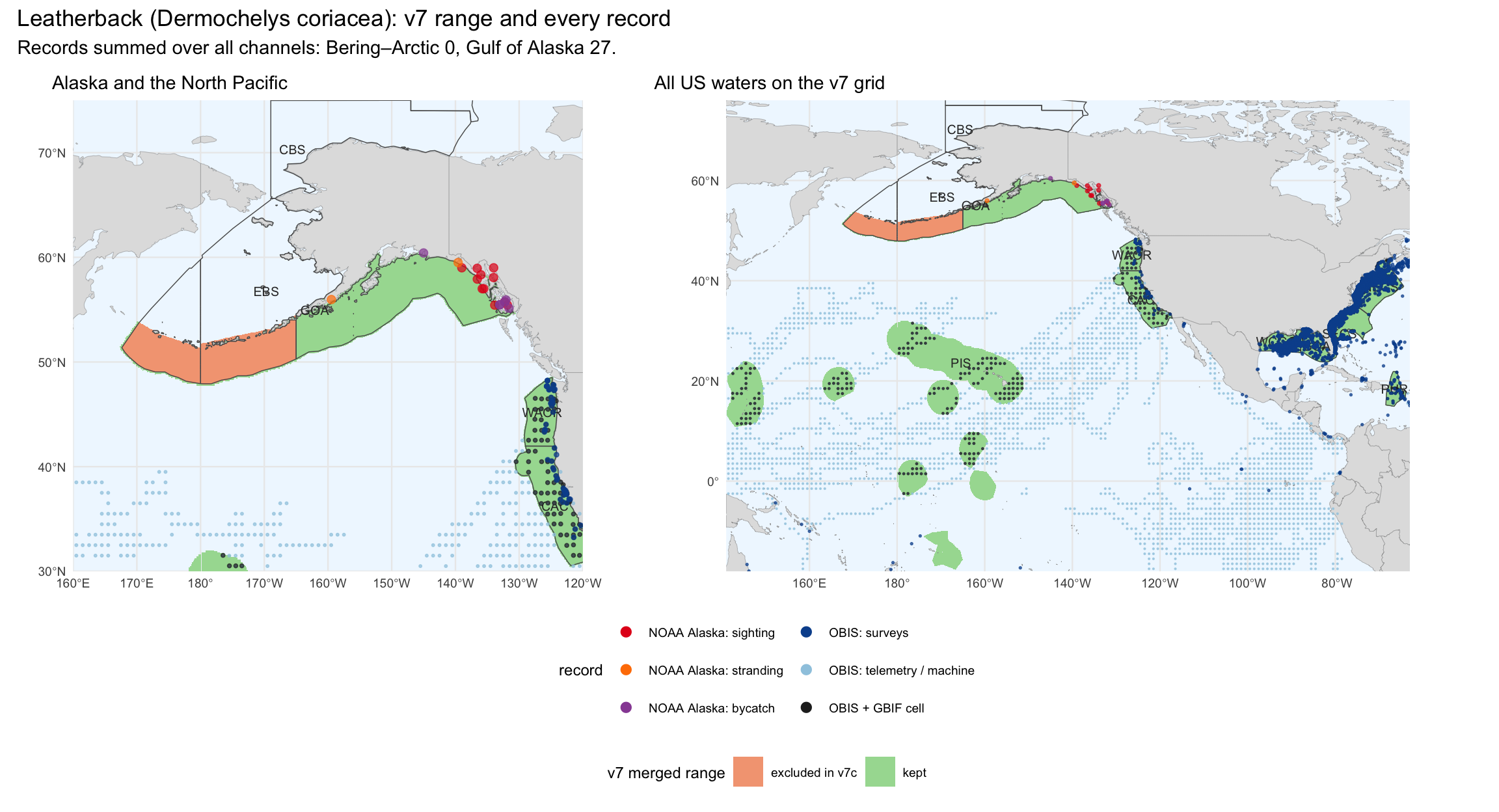
The Bering and Arctic ecoregions are empty for every turtle in every channel. Alaska's channels per
ecoregion, laid side by side:
```{r}
#| label: records-alaska
d_rec |>
filter(eco %in% ECO_AK, aphia %in% d_tu$aphia, covers) |>
select(eco, channel, common, n) |>
pivot_wider(names_from = common, values_from = n) |>
arrange(match(eco, ECO_AK), match(channel, CHANNELS$channel)) |>
kable(caption = "Alaska: sea turtle records per ecoregion and channel (leatherback-only report channels are blank for the other species).")
```
## Looking against finding
A zero only means something where somebody was looking. Per region and channel: the looking (the
channel's effort proxy), the turtles found (any sea turtle), and turtles per 1,000 units of looking.
Lines A–D are the explore notebook's (`data/turtle_encounter/encounter_rates_programarea.csv`); the
GBIF, iNaturalist and OBIS rows are this notebook's whole-ecoregion counts.
```{r}
#| label: looking-finding
d_ep <- read_csv(glue("{dir_te_d}/encounter_rates_programarea.csv")) |>
filter(line != "B+. all records + NOAA AK") |>
mutate(region = recode(grp, "Alaska: Bering to Arctic" = REGION[1], "Alaska: Gulf of Alaska" = REGION[2],
"Pacific (CA/OR/WA)" = REGION[3]),
effort = recode(line,
"A. surveys" = "OBIS turtle-recording surveys: 0.5° block-years searched",
"B. all records" = "OBIS + GBIF: 0.05° cells with a marine mammal record",
"C. public reports" = "iNaturalist (1° coastal buffer): marine mammal + turtle observations",
"D. strandings" = "marine mammal strandings, same coast (Washington for the Pacific)"),
channel = line) |>
select(region, channel, effort, n_effort = n, n_turtle = x)
# the whole-ecoregion channels of this notebook
mm_obis <- open_dataset(f_mega) |>
filter(class == "Mammalia") |> select(cell_id, n) |> collect() |>
inner_join(zc_eco, by = "cell_id") |>
mutate(region = region_of(eco)) |> filter(!is.na(region)) |>
group_by(region) |> summarize(n_effort = sum(n))
tu_obis <- d_obis |>
filter(family %in% FAM_TURTLE) |>
mutate(region = region_of(eco)) |> filter(!is.na(region)) |>
group_by(region) |> summarize(n_turtle = n())
gbif_reg <- function(ds) {
d_gbif |>
filter(dataset == ds, what %in% c("turtle", "mm")) |>
mutate(region = region_of(eco)) |> filter(!is.na(region)) |>
group_by(region, what) |> summarize(n = sum(n), .groups = "drop") |>
pivot_wider(names_from = what, values_from = n) |>
transmute(region, n_effort = mm, n_turtle = turtle)
}
d_lf <- bind_rows(
d_ep,
left_join(mm_obis, tu_obis, by = "region") |>
mutate(channel = "OBIS, all", effort = "OBIS marine mammal records"),
gbif_reg("gbif") |> mutate(channel = "GBIF, all", effort = "GBIF marine mammal records (0.1° ecoregion buffer)"),
gbif_reg("inat") |> mutate(channel = "iNaturalist", effort = "iNaturalist marine mammal observations (0.1° ecoregion buffer)"),
tibble(region = REGION[1:2], channel = "Alaska fishery observers 2014–15",
effort = "observed federal groundfish hauls, Bering Sea–Aleutians and Gulf of Alaska", n_effort = NA, n_turtle = 0L)) |>
mutate(
n_turtle = coalesce(as.integer(n_turtle), 0L),
rate = 1000 * n_turtle / n_effort,
region = factor(region, REGION))
write_csv(d_lf, glue("{dir_out}/looking_vs_finding.csv"), na = "")
d_lf |>
mutate(cell = case_when(
is.na(n_effort) ~ glue("{comma(n_turtle)} turtles"),
n_effort == 0 ~ "not searched",
.default = glue("{comma(n_turtle)} / {comma(n_effort)}<br>{signif(rate, 2)} per 1,000"))) |>
select(channel, effort, region, cell) |>
arrange(region) |>
pivot_wider(names_from = region, values_from = cell) |>
arrange(channel) |>
kable(escape = F, caption = "Looking against finding: turtles / looking, and turtles per 1,000 units of looking, by region.")
```
Bering to Arctic is the only region with a large amount of looking (tens of thousands of marine
mammal records and thousands of searched cells) and no turtle on any channel.
## The exclusion table
```{r}
#| label: exclusions
d_ex_tu <- d_tot |>
filter(aphia %in% d_tu$aphia, eco %in% ECO_AK, n_records == 0) |>
left_join(select(d_sp, aphia, mdl_seq, common_name), by = "aphia") |>
mutate(n_cells_v7 = map2_int(mdl_seq, eco, v7n)) |>
filter(n_cells_v7 >= 1)
ev_tu <- function(a, e) {
d <- d_rec |> filter(aphia == a, eco == e, covers)
glue("0 records in {nrow(d)} channels ({paste(d$channel, collapse = ', ')}); ",
"looking in Bering–Arctic: {comma(d_lf$n_effort[d_lf$channel == 'B. all records' & d_lf$region == REGION[1]])} ",
"OBIS+GBIF cells with a marine mammal record, {comma(d_lf$n_effort[d_lf$channel == 'GBIF, all' & d_lf$region == REGION[1]])} ",
"GBIF marine mammal records")
}
rw_gulf <- d_rec |> filter(aphia == RW$aphia, eco %in% ECO_GULF, covers)
rw_atl <- d_rec |> filter(aphia == RW$aphia, eco %in% ECO_ATL, covers)
ev_rw <- function(e) {
g <- rw_gulf |> filter(eco == e)
glue("{e}: OBIS {g$n[g$channel == 'obis_all']} records, GBIF {g$n[g$channel == 'gbif']}, ",
"OBIS+GBIF cells {g$n[g$channel == 'speciesgrids']}; Atlantic (NECS+SECS): OBIS ",
"{comma(sum(rw_atl$n[rw_atl$channel == 'obis_all']))}, GBIF {comma(sum(rw_atl$n[rw_atl$channel == 'gbif']))}; ",
"no critical habitat in the Gulf; Roberts et al. (2016) model the species in the Atlantic only")
}
d_ex <- bind_rows(
d_ex_tu |>
transmute(mdl_seq, taxon_id = aphia, common_name, zone_fld = "ecoregion_key", zone_key = eco, n_cells_v7,
n_records = n_records, reason = "never recorded",
evidence = map2_chr(aphia, eco, ev_tu)),
tibble(eco = ECO_GULF) |>
transmute(mdl_seq = RW$mdl_seq, taxon_id = RW$aphia, common_name = RW$common_name, zone_fld = "ecoregion_key",
zone_key = eco, n_cells_v7 = map_int(eco, \(e) v7n(RW$mdl_seq, e)),
n_records = map_int(eco, \(e) sum(rw_gulf$n[rw_gulf$eco == e & rw_gulf$channel %in% c("obis_all", "gbif")])),
reason = "outside range: Gulf of America", evidence = map_chr(eco, ev_rw))) |>
mutate(mdl_seq = as.integer(mdl_seq), taxon_id = as.integer(taxon_id)) |>
arrange(mdl_seq, zone_key)
write_csv(d_ex, glue("{dir_out}/zone_exclusions.csv"))
# the records behind each exclusion ----
n_rw <- function(ecos, ch) sum(d_rec$n[d_rec$aphia == RW$aphia & d_rec$eco %in% ecos & d_rec$channel %in% ch & d_rec$covers])
stopifnot(
"the exclusions table must have 6 rows" = nrow(d_ex) == 6,
"every turtle exclusion has 0 records in every channel" =
all(map2_lgl(d_ex_tu$aphia, d_ex_tu$eco, \(a, e) all(d_rec$n[d_rec$aphia == a & d_rec$eco == e & d_rec$covers] == 0))),
"the turtle exclusions are EBS x loggerhead, green, leatherback, olive ridley" =
setequal(paste(d_ex_tu$mdl_seq, d_ex_tu$eco), paste(c(54238, 54239, 54241, 54243), "EBS")),
"turtle exclusion cell counts" =
identical(d_ex$n_cells_v7[match(c(54238, 54239, 54241, 54243), d_ex$mdl_seq)], c(38064L, 39228L, 39959L, 24228L)),
"right whale exclusion cell counts" =
identical(d_ex$n_cells_v7[d_ex$mdl_seq == 54252], c(5626L, 7291L)), # EGOA, WCGOA
"GOA must keep >= 1 record for each of loggerhead, green, leatherback, olive ridley" =
all(d_tot$n_records[d_tot$eco == "GOA" & d_tot$aphia %in% c(137205, 137206, 137209, 220293)] >= 1),
# a handful in the Gulf against thousands in the Atlantic, channel by channel. OBIS holds 11 Gulf records
# (1963, two in 1994, eight undated), one over the plan's "<= 10", so the bound is a share of the Atlantic
# and a count of 15 per channel
"right whale Gulf records must be <= 15 per channel (OBIS, GBIF, OBIS+GBIF cells)" =
all(map_dbl(c("obis_all", "gbif", "speciesgrids"), \(ch) n_rw(ECO_GULF, ch)) <= 15),
"right whale Gulf records must be < 1 % of the Atlantic's in every channel" =
all(map_dbl(c("obis_all", "gbif", "speciesgrids"), \(ch) n_rw(ECO_GULF, ch) / n_rw(ECO_ATL, ch)) < 0.01),
"right whale Atlantic records (OBIS, GBIF) must be >= 1,000" =
n_rw(ECO_ATL, "obis_all") >= 1000 && n_rw(ECO_ATL, "gbif") >= 1000)
d_ex |>
select(mdl_seq, taxon_id, common_name, zone_key, n_cells_v7, n_records, reason) |>
kable(format.args = list(big.mark = ","), caption = "`data/v7c/zone_exclusions.csv`: what v7c removes.")
```
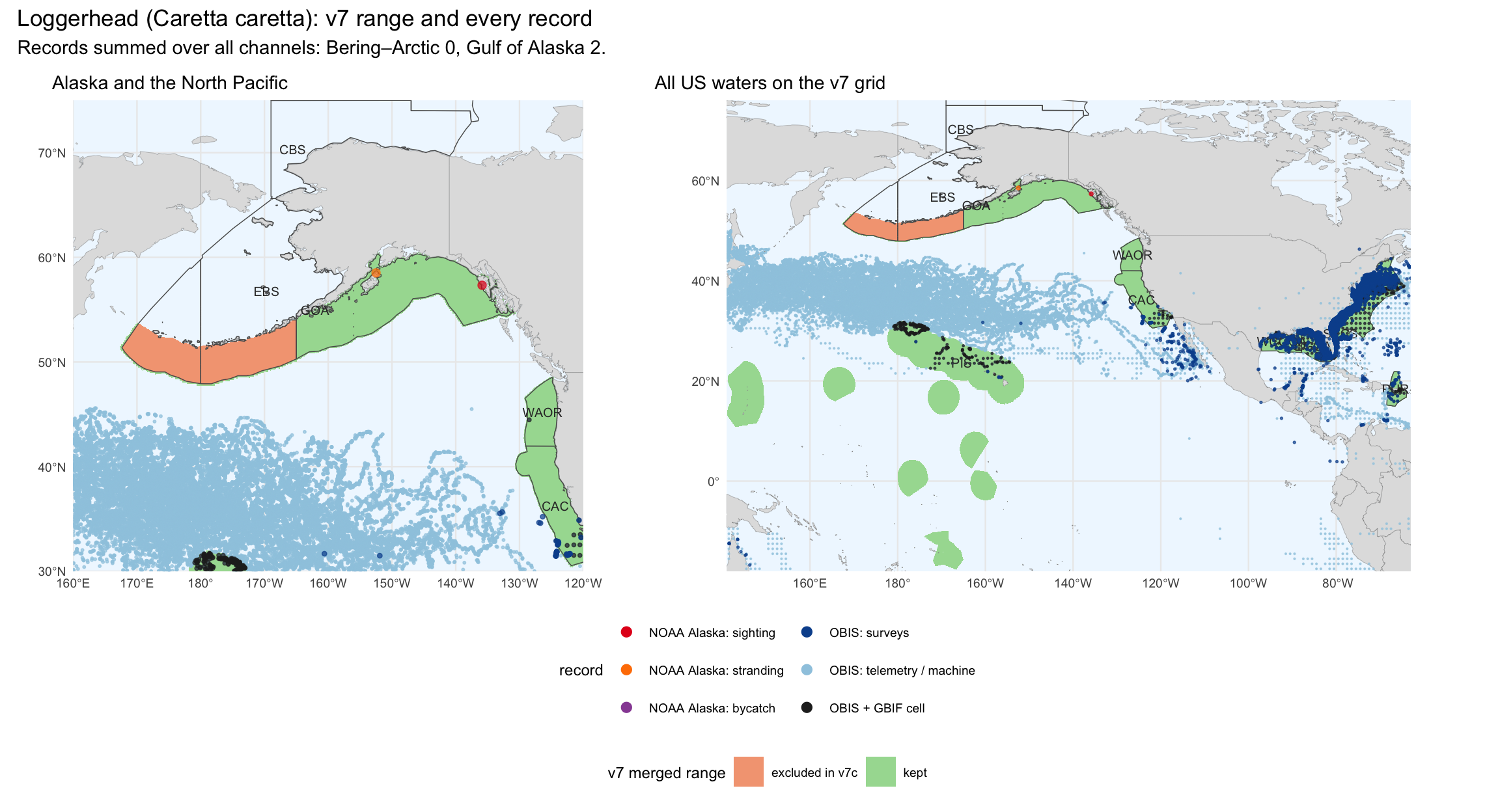
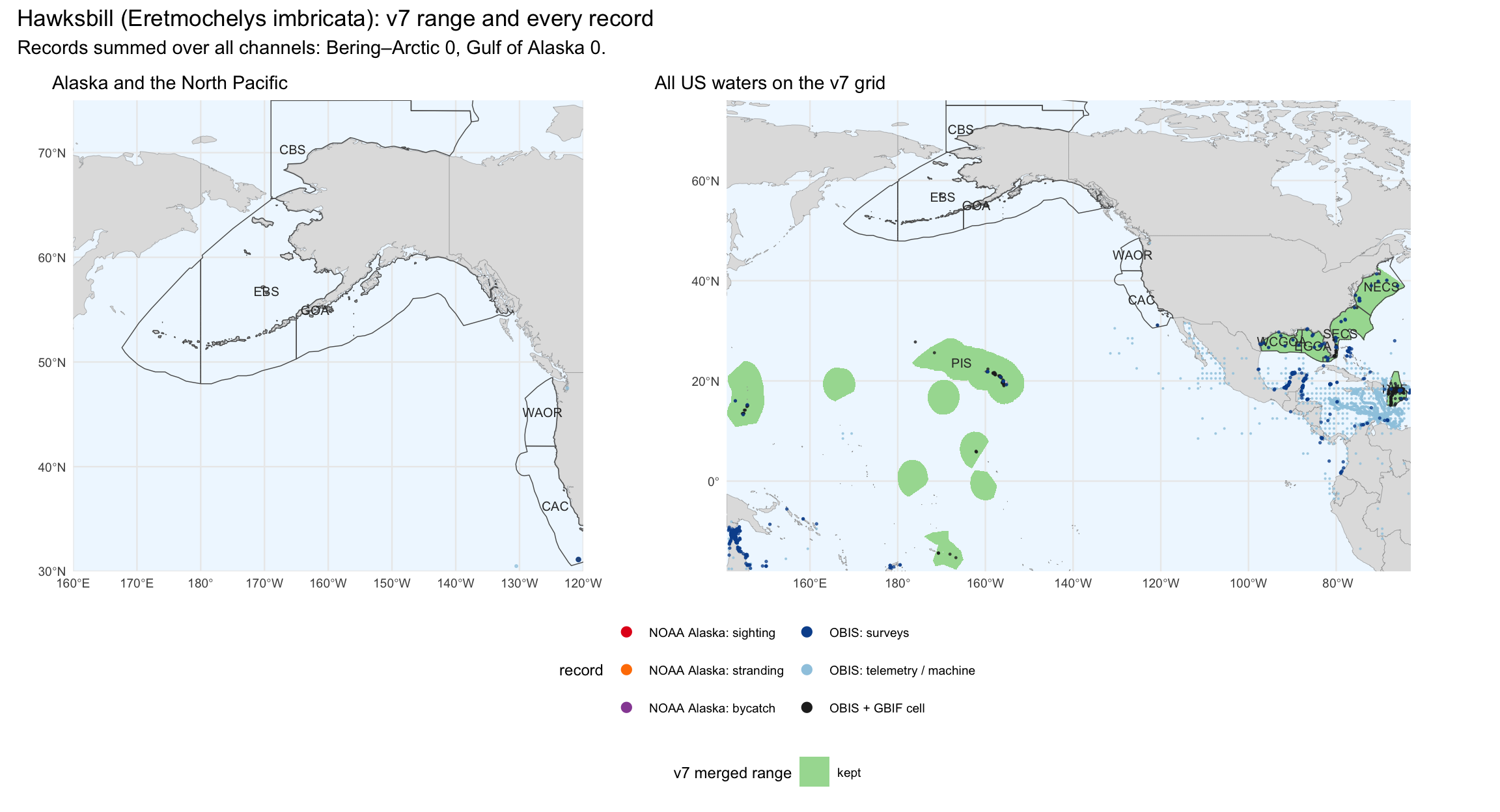
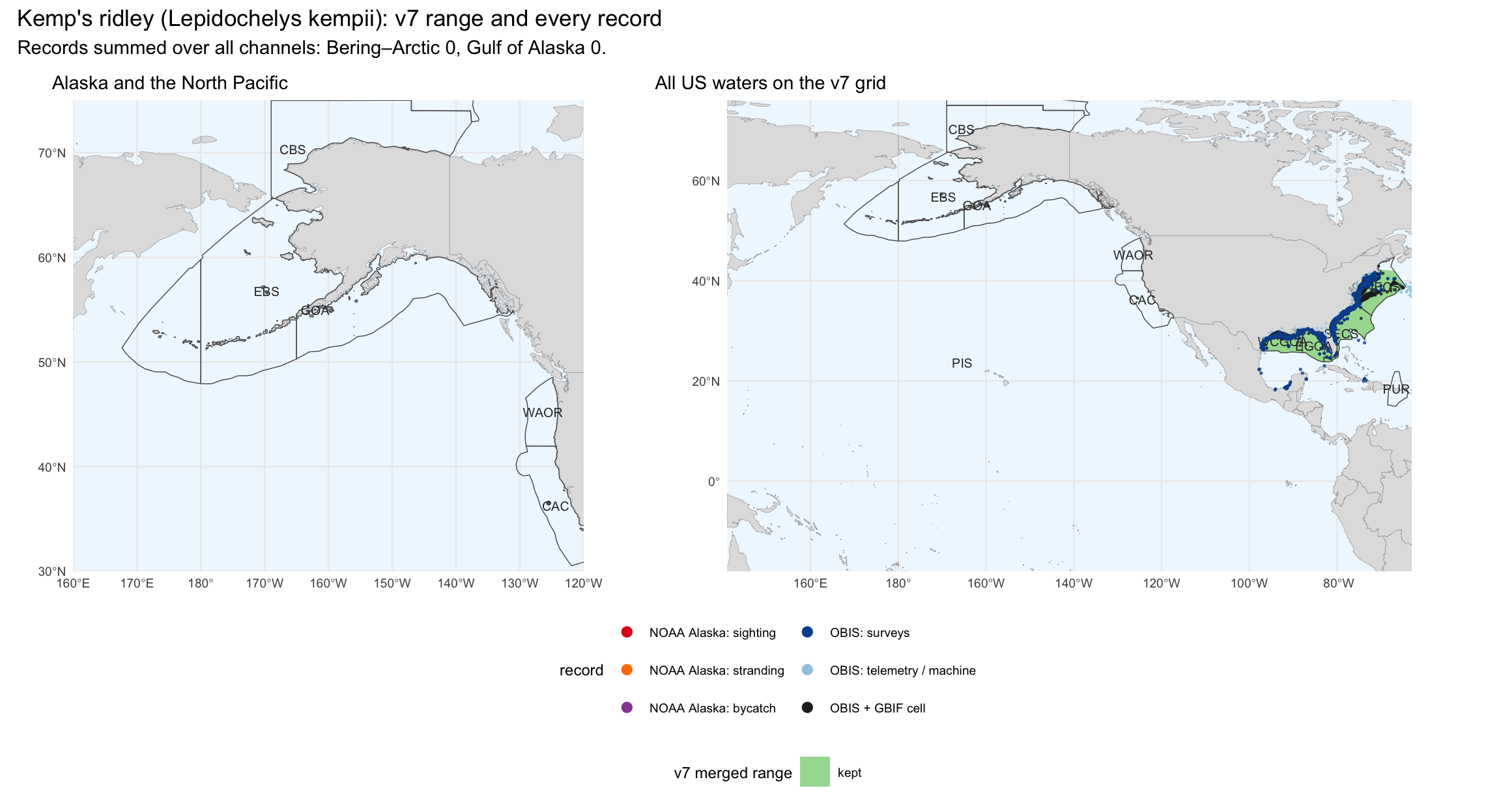
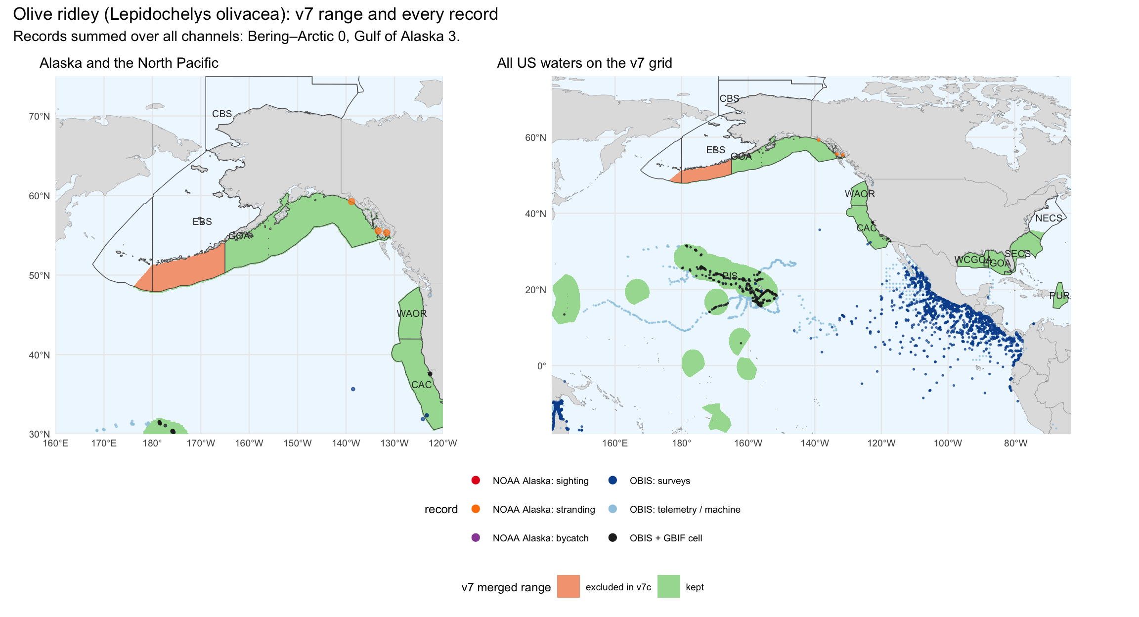
Hawksbill and Kemp's ridley are also never recorded in Alaska, and no turtle in the Chukchi/Beaufort
or High Arctic, but v7 already gives them no range there, so they need no row. The Gulf of Alaska
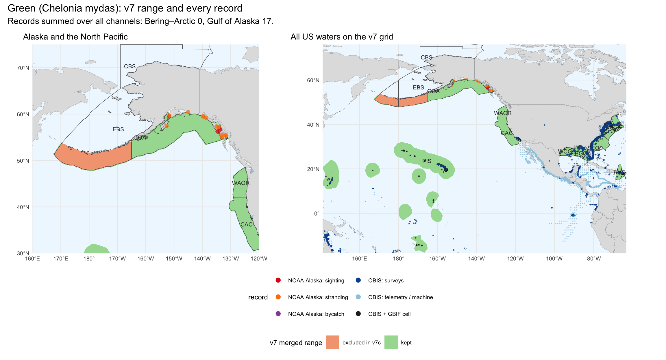
keeps loggerhead, green, leatherback and olive ridley: all four are in the NOAA Alaska file.
## The right whale: Gulf of America against the Atlantic
```{r}
#| label: right-whale
# OBIS published ensemble: cells at or above its 10th-percentile training presence threshold
con <- dbConnect(duckdb())
dbx(con, glue("ATTACH '{db_card}' AS card (READ_ONLY)"))
d_p10 <- dbGetQuery(con, glue("
SELECT c.cell_id, p.thr FROM card.og_cell c JOIN card.og_p10 p USING (taxon)
WHERE c.taxon = {RW$aphia} AND c.val >= p.thr"))
dbDisconnect(con, shutdown = T)
r_p10 <- d_p10 |> inner_join(zc_eco, by = "cell_id") |> count(eco, name = "n")
rw_obis_ev <- d_obis |> filter(aphia == RW$aphia, !is.na(eco), eco %in% ECO_GULF) |>
select(eco, lon, lat, year, datasetName, basisOfRecord)
d_rw <- bind_rows(
d_rec |> filter(aphia == RW$aphia, covers) |>
transmute(channel, unit, eco, n, year_first, year_last, source),
r_p10 |> transmute(channel = "obis_sdm_p10", unit = "0.05° cells", eco, n,
source = "obis_sdm2025"),
d_v7n |> filter(mdl_seq == MDL_CH_RW) |>
transmute(channel = "v7_ch_nmfs", unit = "v7 cells", eco, n = n_cells, source = "nmfs_ch"),
d_rw_cell |> filter(ds_key != "ch_nmfs", !is.na(eco)) |> count(ds_key, eco) |>
transmute(channel = paste0("v7_", ds_key), unit = "v7 cells", eco, n, source = "v7"),
# confirmed Gulf sightings named by NOAA's 2006 release (dates and places, not records in any database)
tibble(channel = "noaa_2006_release", unit = "sighting events",
eco = c("EGOA", "WCGOA"), n = c(2L, 1L), year_first = c(1963L, 2006L), year_last = c(2004L, 2006L),
source = "noaa_sero2006")) |>
complete(nesting(channel, unit, source), eco = ECO, fill = list(n = 0L)) |>
mutate(region = case_when(eco %in% ECO_GULF ~ "Gulf of America", eco %in% ECO_ATL ~ "Atlantic",
eco %in% c(ECO_AK, ECO_PAC, "PIS") ~ "Pacific / Alaska", .default = "Caribbean")) |>
select(region, eco, channel, unit, n, year_first, year_last, source)
d_rw <- bind_rows(
d_rw,
d_rw |> filter(region %in% c("Gulf of America", "Atlantic")) |>
group_by(region, eco = if_else(region == "Gulf of America", "EGOA+WCGOA", "NECS+SECS"), channel, unit, source) |>
summarize(n = sum(n), year_first = suppressWarnings(min(year_first, na.rm = T)),
year_last = suppressWarnings(max(year_last, na.rm = T)), .groups = "drop") |>
mutate(across(starts_with("year_"), \(y) as.integer(if_else(is.finite(y), y, NA_real_))))) |>
arrange(match(region, c("Gulf of America", "Atlantic")), eco, channel)
stopifnot(
"OBIS P10 reaches the Gulf" = sum(r_p10$n[r_p10$eco %in% ECO_GULF]) == 0,
"OBIS P10 must reach the Atlantic" = sum(r_p10$n[r_p10$eco %in% ECO_ATL]) > 1000)
write_csv(d_rw, glue("{dir_out}/right_whale_records.csv"), na = "")
d_rw |>
filter(eco %in% c("EGOA+WCGOA", "NECS+SECS")) |>
select(channel, unit, region, n) |>
pivot_wider(names_from = region, values_from = n) |>
kable(format.args = list(big.mark = ","), caption = "North Atlantic right whale: Gulf of America (EGOA + WCGOA) against the Atlantic (NECS + SECS).")
```
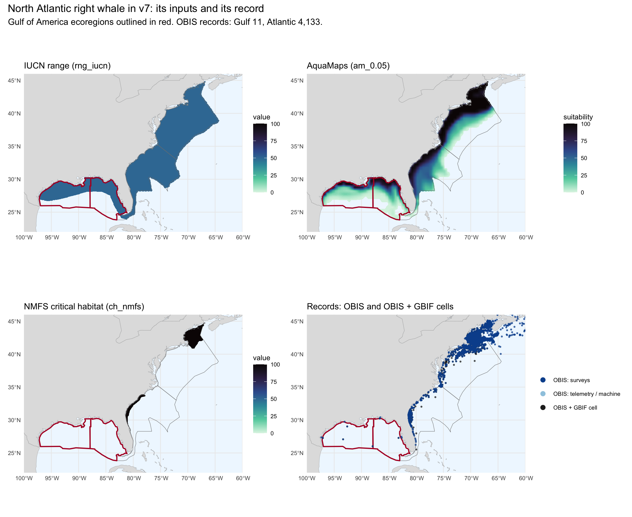
The Gulf holds a handful of records against thousands in the Atlantic, in every channel. OBIS has
`r n_rw(ECO_GULF, "obis_all")`: one from 1963 off Longboat Key (the BLM CETAP compilation), two
from the 1994 SEFSC oceanic survey, and eight undated (Harte Research Institute), listed below.
NOAA's 2006 release names the confirmed Gulf sightings of the time: 1963 off Longboat Key, 2004 off
Panama City, and a mother and calf first seen off Corpus Christi in January 2006 (see also
Ward-Geiger et al. 2011). These are vagrants. The v7 range in the Gulf comes from the IUCN range
polygon (flat value 50) and AquaMaps; critical habitat, the OBIS ensemble at its P10 threshold and
the density model of Roberts et al. (2016) all stop at the Atlantic. GBIF's handful of right whale
records in the Pacific and Arctic (1905, 1916) are old identifications of what is now the North
Pacific right whale, *Eubalaena japonica*; v7 gives the North Atlantic species no range there.
```{r}
#| label: right-whale-obis-gulf
stopifnot(nrow(rw_obis_ev) == n_rw(ECO_GULF, "obis_all"))
rw_obis_ev |> arrange(year) |>
kable(digits = 2, caption = "The OBIS right whale records in the Gulf of America.")
```
## Figures
```{r}
#| label: fig-prep
# land and ecoregion outlines in 0-360 longitude, so Alaska is not split at the antimeridian
land <- ne_countries(scale = 50, returnclass = "sf") |>
st_make_valid() |>
st_break_antimeridian(lon_0 = 180) |>
st_shift_longitude() |> select(geometry)
ln_eco <- ply_eco |>
st_cast("MULTILINESTRING") |> st_break_antimeridian(lon_0 = 180) |>
st_shift_longitude() |> st_simplify(dTolerance = 0.05)
lbl_eco <- ply_eco |> st_break_antimeridian(lon_0 = 180) |> st_shift_longitude() |>
st_cast("POLYGON") |> mutate(a = as.numeric(st_area(geom))) |>
group_by(eco) |> slice_max(a, n = 1, with_ties = F) |> ungroup() |> st_point_on_surface()
lbl_eco <- tibble(eco = lbl_eco$eco, x = st_coordinates(lbl_eco)[, 1], y = st_coordinates(lbl_eco)[, 2])
ex_eco <- d_ex |> distinct(mdl_seq, zone_key)
# record points per species: the NOAA Alaska file and OBIS at their coordinates, speciesgrids at cell centres
x360 <- function(lon) if_else(lon < 0, lon + 360, lon)
CH_LBL <- c(
noaa_ak_sighting = "NOAA Alaska: sighting", noaa_ak_stranding = "NOAA Alaska: stranding",
noaa_ak_bycatch = "NOAA Alaska: bycatch", obis_survey = "OBIS: surveys", obis_other = "OBIS: telemetry / machine",
speciesgrids = "OBIS + GBIF cell")
CH_COL <- c("#e41a1c", "#ff7f00", "#984ea3", "#08519c", "#9ecae1", "#252525") |> set_names(CH_LBL)
CH_SIZE <- c(2, 2, 2, 1, 0.5, 0.8) |> set_names(CH_LBL)
CH_DRAW <- CH_LBL[c(5, 6, 4, 1, 2, 3)] # telemetry at the bottom, the NOAA Alaska file on top
d_pts <- bind_rows(
d_ak |> filter(status == "in Alaska waters", !is.na(aphia)) |>
transmute(aphia, x = x360(lon), y = lat, channel = paste0("noaa_ak_", type)),
d_obis |> filter(aphia %in% d_sp$aphia) |>
transmute(aphia, x = x360(lon), y = lat, channel = if_else(is_survey, "obis_survey", "obis_other")) |>
distinct(),
d_sg |> filter(aphia %in% d_sp$aphia) |> distinct(aphia, cell_id) |>
mutate(g05_xy(cell_id)) |> transmute(aphia, x = x360(lon), y = lat, channel = "speciesgrids")) |>
mutate(channel = factor(CH_LBL[channel], CH_LBL))
FRAME_AK <- list(x = c(160, 240), y = c(30, 75)) # North Pacific, Alaska to California
FRAME_US <- list(x = c(141, 297), y = c(-18, 76)) # the v7 grid
map_turtle <- function(i) {
sp <- d_tu[i, ]
rng <- d_tu_cell |> filter(mdl_seq == sp$mdl_seq) |>
mutate(v7_xy(cell_id),
status = if_else(paste(mdl_seq, eco) %in% paste(ex_eco$mdl_seq, ex_eco$zone_key), "excluded in v7c", "kept"))
pts <- d_pts |> filter(aphia == sp$aphia)
panel <- function(fr, title, pt_size) {
pts_f <- pts |> filter(between(x, fr$x[1], fr$x[2]), between(y, fr$y[1], fr$y[2]))
ggplot() +
geom_raster(data = rng, aes(x, y, fill = status)) +
geom_sf(data = land, fill = "grey88", color = "grey60", linewidth = 0.1) +
geom_sf(data = ln_eco, color = "grey35", linewidth = 0.25) +
geom_text(data = lbl_eco, aes(x, y, label = eco), size = 2.6, color = "grey20") +
geom_point(data = arrange(pts_f, match(channel, CH_DRAW)), aes(x, y, color = channel, size = channel), alpha = 0.7, show.legend = c(colour = T, fill = F, size = F)) +
scale_fill_manual(values = c(kept = "#a6dba0", `excluded in v7c` = "#f4a582"), drop = F, name = "v7 merged range") +
scale_color_manual(values = CH_COL, drop = F, name = "record") +
scale_size_manual(values = pt_size * CH_SIZE, drop = F, guide = "none") +
guides(color = guide_legend(override.aes = list(size = 2.5, alpha = 1), ncol = 2)) +
coord_sf(xlim = fr$x, ylim = fr$y, expand = F) +
labs(title = title, x = NULL, y = NULL) +
theme_minimal(base_size = 9) + theme(panel.background = element_rect(fill = "aliceblue", color = NA))
}
n_ba <- sum(d_tot$n_records[d_tot$aphia == sp$aphia & d_tot$eco %in% ECO_BA])
n_goa <- d_tot$n_records[d_tot$aphia == sp$aphia & d_tot$eco == "GOA"]
(panel(FRAME_AK, "Alaska and the North Pacific", 1) | panel(FRAME_US, "All US waters on the v7 grid", 0.4)) +
plot_layout(guides = "collect", widths = c(1, 1.5)) +
plot_annotation(
title = glue("{sp$common} ({sp$sci}): v7 range and every record"),
subtitle = glue("Records summed over all channels: Bering–Arctic {n_ba}, Gulf of Alaska {n_goa}.")) &
theme(legend.position = "bottom", legend.box = "vertical")
}
```
### Sea turtles
Each species' v7 merged range (green: kept; orange: excluded in v7c) with every record that has a
place: the NOAA Alaska file and OBIS at their coordinates, OBIS + GBIF (`speciesgrids`, which carries
the iNaturalist records) at cell centres. Records outside the US grid are cut by the frame.
```{r}
#| label: fig-turtles
#| fig-width: 12
#| fig-height: 6.5
for (i in seq_len(nrow(d_tu))) {
p <- map_turtle(i)
ggsave(glue("{dir_img}/turtle_{d_tu$sp_key[i]}_records.png"), p, width = 12, height = 6.5, dpi = 150, bg = "white")
print(p)
}
```
### North Atlantic right whale
```{r}
#| label: fig-right-whale
#| fig-height: 9
#| fig-width: 11
FRAME_RW <- list(x = c(260, 300), y = c(22, 46))
rw_cells <- d_rw_cell |> mutate(v7_xy(cell_id))
ln_gulf <- ln_eco |> filter(eco %in% ECO_GULF)
rw_panel <- function(d, title, fill_lab, pts = NULL) {
p <- ggplot()
if (!is.null(d)) p <- p + geom_raster(data = d, aes(x, y, fill = val)) +
scale_fill_viridis_c(name = fill_lab, option = "mako", direction = -1, limits = c(0, 100))
p <- p +
geom_sf(data = land, fill = "grey88", color = "grey60", linewidth = 0.1) +
geom_sf(data = ln_eco, color = "grey50", linewidth = 0.2) +
geom_sf(data = ln_gulf, color = "#b2182b", linewidth = 0.7)
if (!is.null(pts)) p <- p +
geom_point(data = arrange(pts, match(channel, CH_DRAW)), aes(x, y, color = channel), size = 0.6, alpha = 0.7) +
scale_color_manual(values = CH_COL, name = NULL) +
guides(color = guide_legend(override.aes = list(size = 2.5, alpha = 1)))
p + coord_sf(xlim = FRAME_RW$x, ylim = FRAME_RW$y, expand = F) +
labs(title = title, x = NULL, y = NULL) +
theme_minimal(base_size = 9) + theme(panel.background = element_rect(fill = "aliceblue", color = NA))
}
p_rw <- (
rw_panel(filter(rw_cells, ds_key == "rng_iucn"), "IUCN range (rng_iucn)", "value") |
rw_panel(filter(rw_cells, ds_key == "am_0.05"), "AquaMaps (am_0.05)", "suitability")) /
(rw_panel(filter(rw_cells, ds_key == "ch_nmfs"), "NMFS critical habitat (ch_nmfs)", "value") |
rw_panel(NULL, "Records: OBIS and OBIS + GBIF cells", NULL,
pts = filter(d_pts, aphia == RW$aphia, between(x, 260, 300), between(y, 22, 46)))) +
plot_annotation(
title = "North Atlantic right whale in v7: its inputs and its record",
subtitle = glue("Gulf of America ecoregions outlined in red. OBIS records: Gulf {n_rw(ECO_GULF, 'obis_all')}, ",
"Atlantic {comma(n_rw(ECO_ATL, 'obis_all'))}."))
f_rw_png <- glue("{dir_img}/right_whale_records.png")
ggsave(f_rw_png, p_rw, width = 11, height = 9, dpi = 150, bg = "white")
p_rw
```
### Interactive map
Toggle the layers at the top right: the v7 turtle range (number of species per cell), the right
whale's v7 range, the excluded ecoregions, and the records by channel (thinned to one point per
0.1° per channel and species group).
```{r}
#| label: map-interactive
# v7 range rasters on the v7 grid (0-360): turtle species per cell, right whale presence
r_tu <- rast(r_v7); r_tu[] <- NA
n_tu <- d_tu_cell |> count(cell_id)
r_tu[n_tu$cell_id] <- n_tu$n
r_tu <- trim(r_tu)
TU_COLS <- c("#edf8e9", "#c7e9c0", "#a1d99b", "#74c476", "#31a354", "#006d2c")
coltab(r_tu) <- data.frame(value = 1:6, t(col2rgb(TU_COLS, alpha = T)))
r_rwm <- rast(r_v7); r_rwm[] <- NA
r_rwm[filter(d_rw_cell, ds_key == "ms_merge")$cell_id] <- 1L
r_rwm <- trim(r_rwm)
coltab(r_rwm) <- data.frame(value = 1, t(col2rgb("#6a51a3", alpha = T)))
ply_ex <- bind_rows(
ply_eco |> filter(eco == "EBS") |> mutate(what = "turtles excluded: East Bering Sea"),
ply_eco |> filter(eco %in% ECO_GULF) |> mutate(what = glue("right whale excluded: {eco_name}"))) |>
st_break_antimeridian(lon_0 = 180) |> st_shift_longitude() |> st_simplify(dTolerance = 0.02)
pts_map <- d_pts |>
filter(!is.na(channel), between(x, FRAME_US$x[1], FRAME_US$x[2]), between(y, FRAME_US$y[1], FRAME_US$y[2])) |>
mutate(grp = if_else(aphia == RW$aphia, "right whale", "sea turtle"),
x = floor(x / 0.1) * 0.1 + 0.05, y = floor(y / 0.1) * 0.1 + 0.05) |>
distinct(grp, channel, x, y) |>
st_as_sf(coords = c("x", "y"), crs = 4326, remove = F)
m <- maplibre(style = carto_style("positron"), center = c(-140, 45), zoom = 2, height = "620px",
cooperativeGestures = T) |>
add_image_source(id = "tu_src", data = r_tu) |>
add_raster_layer(id = "v7 turtle range (species per cell)", source = "tu_src",
raster_resampling = "nearest", raster_opacity = 0.75) |>
add_image_source(id = "rw_src", data = r_rwm) |>
add_raster_layer(id = "v7 right whale range", source = "rw_src", raster_resampling = "nearest",
raster_opacity = 0.5, visibility = "none") |>
add_fill_layer(id = "excluded in v7c", source = ply_ex, fill_color = "#d6604d", fill_opacity = 0.25,
fill_outline_color = "#b2182b", tooltip = "what")
lyr_ids <- c("v7 turtle range (species per cell)", "v7 right whale range", "excluded in v7c")
for (g in c("sea turtle", "right whale")) for (ch in levels(pts_map$channel)) {
d <- filter(pts_map, grp == g, channel == ch)
if (nrow(d) == 0) next
id <- glue("{g}: {ch}")
m <- m |> add_circle_layer(
id = id, source = d, circle_color = CH_COL[[ch]], circle_radius = 3, circle_opacity = 0.75,
circle_stroke_color = if (g == "right whale") "#000000" else "#ffffff", circle_stroke_width = 0.5,
tooltip = "channel")
lyr_ids <- c(lyr_ids, id)
}
m |>
add_layers_control(layers = lyr_ids, collapsible = T, position = "top-right") |>
mapgl::add_legend("turtle species in v7 range", values = 1:6, colors = TU_COLS, type = "categorical",
position = "bottom-left") |>
add_fullscreen_control(position = "top-left") |>
add_navigation_control() |>
add_scale_control()
```
## Sources
`data/v7c/sources.csv`: every channel used, every report cited, and every request still open. The
citation keys are for the docs' `references.bib`.
```{r}
#| label: sources
d_src <- tribble(
~channel, ~records, ~coverage, ~years, ~effort_proxy, ~citation_key, ~url, ~status,
"noaa_ak_sighting / _stranding / _bycatch",
"Alaska sea turtle records typed by how found (sighting at sea, stranding, netted)", "Alaska (all located records in the Gulf of Alaska)", "1963–2020",
"marine mammal strandings, Alaska Region: 188 a year 2006–2017", "noaa_ak_turtles_2026; hodge_wing2000",
"https://www.fisheries.noaa.gov/feature-story/sea-turtles-alaska-yes-we-have-them-far-north", "used",
"obis_all / obis_survey",
"OBIS presence records (surveys = no telemetry, machine observation or photo-ID)", "global", "1850s–2024",
"OBIS marine mammal records; turtle-recording datasets' block-years", "obis2025",
"https://obis.org/data/access/", "used",
"gbif",
"GBIF presence records, occurrence API counts per ecoregion (0.1° buffer)", "global", "to 2026",
"GBIF marine mammal records", "gbif2026", "https://api.gbif.org/v1/occurrence/search", "used",
"inat",
"iNaturalist research-grade observations via GBIF", "global", "about 2008–2026",
"iNaturalist marine mammal observations", "inaturalist2026",
"https://www.gbif.org/dataset/50c9509d-22c7-4a22-a47d-8c48425ef4a7", "used",
"speciesgrids",
"OBIS + GBIF records merged onto the 0.05° grid (cells)", "global", "undated",
"0.05° cells with a marine mammal record", "speciesgrids2025", "https://github.com/MarineSensitivity/workflows", "used",
"wdfw_wa",
"every Washington sea turtle record (stranding, bycatch, at sea, aerial), Appendix A", "Washington", "1950–2013",
"marine mammal strandings, Washington: 578 a year 2007–2016", "wdfw2017",
"https://wdfw.wa.gov/publications/01870", "used",
"stssn",
"sea turtle strandings by state, species and encounter type (preliminary data application)", "Gulf (TX–FL) and Atlantic (FL–ME)", "2016–2025",
"marine mammal strandings, Gulf: 375 a year 2000–2014 (Litz 2015)", "stssn2026",
"https://connect.fisheries.noaa.gov/content/cb3f4647-9e4f-4f3d-9edf-e7a87a1feef6/", "used",
"wc_groundfish_observer",
"West Coast Groundfish Observer Program: 1 leatherback killed (2008, open-access pot) and 4 seen (2005, 2007, 2011, 2014); the only observed leatherback take", "CA/OR/WA", "2002–2019",
"observer coverage 3–12 % (open-access fixed gear) to 100 % (catch shares)", "benson2026",
"https://doi.org/10.25923/px0e-gh24", "cited",
"wc_leatherback_strandings",
"leatherback strandings: AK 7, WA 9, OR 1, CA 113; none in Alaska since 1993", "AK, WA, OR, CA", "1963–2020",
"", "benson2026", "https://doi.org/10.25923/px0e-gh24", "cited",
"ak_fishery_observer",
"'No sea turtles were observed caught in 2014 or 2015 in Alaska Region fisheries under federal or joint federal/international management authority' (§5.6)", "Bering Sea–Aleutians, Gulf of Alaska", "2014–2015",
"North Pacific Observer Program coverage of federal groundfish and halibut fisheries", "benaka2019",
"https://media.fisheries.noaa.gov/dam-migration/nbr_update_3.pdf", "cited",
"hi_longline_observer",
"Hawaii shallow-set longline, 100 % observer coverage: 46 sea turtle interactions in 2025 (35 loggerhead, 10 leatherback, 1 unidentified hardshell); the fleet fishes mostly outside the EEZ, so not placed in an ecoregion", "Hawaii-based fleet, mostly high seas", "2025",
"59 observed departures", "piro2026",
"https://www.fisheries.noaa.gov/resource/data/hawaii-shallow-set-longline-fishery-quarterly-and-annual-status-report-2025", "cited",
"right whale: noaa_2006_release",
"confirmed Gulf right whale sightings: 1963 Longboat Key, 2004 Panama City, 2006 mother and calf off Corpus Christi", "Gulf of America", "1963–2006",
"", "noaa_sero2006; ward_geiger2011", "https://doi.org/10.18785/goms.2901.06", "cited",
"right whale: density model",
"habitat-based density models from line-transect surveys; the right whale is modelled in the Atlantic only", "US Atlantic and Gulf", "1992–2014",
"aerial and shipboard line-transect effort", "roberts2016", "https://doi.org/10.1038/srep22615", "cited",
"right whale: obis_sdm_p10",
"OBIS published SDM ensemble cells at or above the 10th-percentile training presence threshold", "global", "",
"", "obis_sdm2025", "https://github.com/MarineSensitivity/workflows", "used",
"request 1: NOAA Alaska Region (Jenna Malek)",
"Alaska sea turtle records 2003 to present, typed as the 1963–2020 file; Alaska marine mammal strandings per year by area", "Alaska", "2003–present",
"", "", "", "requested",
"request 2: NOAA West Coast Region stranding coordinators",
"sea turtle strandings per year by state and species, ideally 1980 to present; marine mammal strandings by state", "CA, OR, WA", "1980–present",
"", "", "", "requested",
"request 3: STSSN state coordinators",
"permission to cite the preliminary Gulf and Atlantic counts used here (data release policy)", "Gulf, Atlantic", "2016–2025",
"", "stssn2026", "", "requested",
"request 4: AFSC Marine Mammal Laboratory / Platforms of Opportunity / North Pacific Observer Program",
"any sea turtle record from Alaska cetacean surveys, Platforms of Opportunity (1950–present, non-public) and the observer database, with effort", "Alaska", "1950–present",
"", "", "https://www.fisheries.noaa.gov/inport/item/17407", "requested",
"request 5: SEFSC on-effort database (Lance Garrison)",
"on-effort turtle sightings per km surveyed, Gulf and Atlantic", "Gulf, Atlantic", "",
"", "", "", "requested")
write_csv(d_src, glue("{dir_out}/sources.csv"))
d_src |> select(channel, coverage, years, citation_key, status) |> kable(caption = "`data/v7c/sources.csv`")
```
## Checks
```{r}
#| label: check-outputs
f_out <- glue("{dir_out}/{c('records_species_ecoregion', 'zone_exclusions', 'right_whale_records', 'sources', 'gbif_counts', 'looking_vs_finding')}.csv")
stopifnot(all(file_exists(f_out)), length(dir_ls(dir_img, glob = "*.png")) == 7)
# zone_exclusions.csv read back as build_v7c.qmd will read it
d_chk <- read_csv(glue("{dir_out}/zone_exclusions.csv"))
stopifnot(
nrow(d_chk) == 6, !anyNA(d_chk[c("mdl_seq", "zone_key")]), all(d_chk$zone_fld == "ecoregion_key"),
all(d_chk$zone_key %in% ECO), sum(d_chk$n_cells_v7) == 38064 + 39228 + 39959 + 24228 + 5626 + 7291)
cat(glue("rendered in {round(as.numeric(difftime(Sys.time(), t_start, units = 'mins')), 1)} min"))
```