Ingest Primary Productivity

librarian::shelf(
  cmocean, dplyr, DT, fs, ggplot2, glue, here, htmltools, janitor, jsonlite, leaflet, 
  leaflet.extras, lubridate, mapview, R.utils, readr, sf, stringr, stars, terra, tibble, 
  tidyr, units,
  quiet = T)

yrs         <- 2014:2023  # vgpm-viirs most recent complete 10 years
dir_data    <- "~/My Drive/projects/msens/data"
dir_vgpm    <- glue("{dir_data}/raw/oregonstate.edu/vgpm.r2022.v.chl.v.sst.2160x4320")
vgpm_tif    <- glue("{dir_vgpm}_{min(yrs)}-{max(yrs)}.avg.sd.tif")
vgpm_pa_tif <- glue("{dir_vgpm}_{min(yrs)}-{max(yrs)}.avg.sd_planareas.tif")
vgpm_csv    <- glue("{dir_vgpm}_{min(yrs)}-{max(yrs)}_planareas.avg.sd.csv")


dir_raw     <- glue("{dir_data}/raw/boem.gov")
dir_out     <- glue("{dir_data}/derived")
oa_new_geo  <- glue("{dir_raw}/OCS_Area_Polygons.geojson")
pa_new_geo  <- glue("{dir_raw}/OCS_Proposed_Planning_Area_Polygons.geojson")
pa_oa_geo   <- glue("{dir_out}/pa_oa_2025.geojson")

pa_gpkg     <- glue("{dir_data}/derived/ply_planareas_2025.gpkg")
dir_figs    <- here("figs/ingest_productivity")

verbose    <- F

1 Vertically Generalized Production Model (VGPM), CAFE VIIRS 2014 to 2023 | OregonState

Source:

• Ocean Productivity from Oregon State

• VIIRS R2022 - 2160 by 4320 Monthly HDF files

• old: CAFE model description

• old: Online updated CAFE data

• Silsbe et al (2025) Global declines in net primary production in the ocean color era | Nature Communications. Nature Communications

  • Silsbe et al (2016) The CAFE model: A net production model for global ocean phytoplankton. Global Biogeochemical Cycles

    The Carbon, Absorption, and Fluorescence Euphotic-resolving (CAFE) net primary production model is an adaptable framework for advancing global ocean productivity assessments by exploiting state-of-the-art satellite ocean color analyses and addressing key physiological and ecological attributes of phytoplankton.

    • older: Standara VGPM: 1080 by 2160 Monthly HDF files from VIIRS R2022
    • Frequently Asked Questions

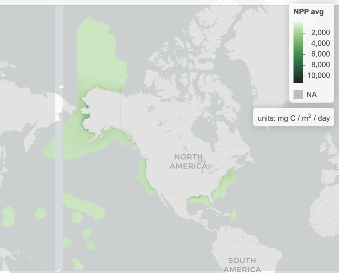
Calculated sum of 2014 to 2023 monthly net primary production (NPP) from VIIRS data.

Community guidance for developing this website was to provide a single productivity product as a Standard product. For this, we initially chose the original Vertically Generalized Production Model (VGPM) (Behrenfeld and Falkowski, 1997a) as the standard algorithm. The VGPM is a “chlorophyll-based” model that estimate net primary production from chlorophyll using a temperature-dependent description of chlorophyll-specific photosynthetic efficiency. For the VGPM, net primary production is a function of chlorophyll, available light, and the photosynthetic efficiency.

Standard products are based on chlorophyll, temperature and PAR data from SeaWiFS, MODIS and VIIRS satellites, along with estimates of euphotic zone depth from a model developed by Morel and Berthon (1989) and based on chlorophyll concentration.

Units: mg C / m² / day

Citation: Behrenfeld and Falkowski, 1997a

• Ocean Productivity: Online updated CAFE data

if (!file.exists(vgpm_tif)) {
  
  for (yr in yrs){ # yr = 2015
    
    # vgpm_yr_tif  <- glue("{dir_vgpm}/cafe.v.{yr}.tif")
    vgpm_yr_tif  <- glue("{dir_vgpm}/vgpm.{yr}.tif")
    
    if (!file.exists(vgpm_yr_tif)) {
      tar      <- glue("vgpm.v.{yr}.tar")
      url_tar  <- glue("https://orca.science.oregonstate.edu/data/2x4/monthly/vgpm.r2022.v.chl.v.sst/hdf/{tar}")
      path_tar <- file.path(dir_vgpm, tar)
      
      dir_create(dirname(path_tar))
      if(!file_exists(path_tar))
        download.file(url_tar, path_tar, method = "curl", extra = "-k -L")
      
      dir_untar <- path_ext_remove(path_tar)
      dir_create(dir_untar)
      untar(path_tar, exdir = dir_untar)
      
      # Get list of compressed files
      files_gz <- dir_ls(dir_untar, glob = "*.gz")
      
      dir_unzip <- path(dir_untar, "unzipped")
      dir_create(dir_unzip)
      
      # Unzip all files
      for (file_gz in files_gz) { # file_gz = files_gz[1]
        file_hdf <- path(dir_unzip, sub("\\.gz$", "", basename(file_gz)))
        
        if (!file.exists(file_hdf))
          gunzip(file_gz, destname = file_hdf)
      }
      
      # Get list of unzipped HDF files
      files_hdf <- dir_ls(dir_unzip, glob = "*.hdf") # length(files_hdf) = 12
      
      # Function to read VGPM data from HDF file
      read_vgpm_hdf <- function(file_hdf) { # file_hdf <- files_hdf[7]
        # First, query the HDF file to see the subdatasets
        # file_exists(file_hdf)
        
        r <- read_stars(file_hdf) |> # read all subdatasets
          rast()
        ext(r) <- c(-180, 180, -90, 90) # set extent to global
        crs(r) <- "epsg:4326"
        NAflag(r) <- -9999
        names(r) <- "npp" # set name for all layers
        
        time(r, tstep = "yearmonths") <- basename(file_hdf) |> 
          str_replace("vgpm.([0-9]+).hdf", "\\1") |>
          as_date(format = "%Y%j")
        
        r
      }
      
      # Initialize a list to store all monthly rasters
      monthly_rasters <- list()
      
      # Read all monthly files
      for (i in seq_along(files_hdf)) {
        if (verbose)
          message("Processing file", i, "of", length(files_hdf), ":", files_hdf[i], "\n")
        r <- read_vgpm_hdf(files_hdf[i])
        
        if (!is.null(r)) {
          monthly_rasters[[i]] <- r
        }
      }
      
      # Create a SpatRaster collection from all the monthly rasters
      r_yr <- rast(monthly_rasters) |> 
        mean(na.rm = T)
      names(r_yr) <- "npp"
      time(r_yr, tstep = "years") <- yr

      writeRaster(r_yr, vgpm_yr_tif, overwrite = TRUE)
      
      dir_delete(dir_untar)
      file_delete(path_tar)
      
      message(glue(
        "Created annual for {yr}: {basename(vgpm_yr_tif)}"))
    }
  }
  
  # aggregate across years ----
  r_yrs <- dir_ls(dir_vgpm, glob = "*.tif") |> 
    rast()
  
  r_avg <- r_yrs |> 
    mean(na.rm = T)

  r_sd <- r_yrs |> 
    stdev(na.rm = T)
    
  r <- c(r_avg, r_sd) |> 
    setNames(glue("npp_{c('avg','sd')}"))
  
  r |> 
    writeRaster(vgpm_tif, overwrite = T)
}

r <- rast(vgpm_tif,  lyrs = "npp_avg")
#   # rotate(left=F) # -180 to 180 -> 0 to 360
#   # shift(dx = 0.0001) # problem with -180 extent

if (!file.exists(vgpm_pa_tif)) {
  
  cell_tif <- glue("{dir_data}/derived/r_bio-oracle_planarea.tif")
  
  r_cell <- rast(cell_tif, lyrs = "cell_id")
  
  # downsample and mask
  r_r <- rotate(r)  # [-180, 180] -> [0, 360]
  
  r_ds <- terra::resample(
    r_r,
    r_cell,
    method = "bilinear") |>
    mask(r_cell) |> 
    crop(r_cell)
  # plot(r_ds, main = "Downsampled Productivity"
  
  writeRaster(r_ds, vgpm_pa_tif, overwrite = T)
}
r_pa <- rast(vgpm_pa_tif)  

vgpm_png <- here("figs/ingest_productivity/map_vgpm_avg.png")
if (!file.exists(vgpm_png)){
  m <- mapView(
    r_pa, maxpixels = ncell(r), col.regions = cmocean("algae"),
    layer.name = glue("NPP avg")) |> 
    slot("map") |>
    # addFullscreenControl() |>
    addControl(tags$div(HTML("units: mg C / m<sup>2</sup> / day")), position = "topright") |> 
    removeMapJunk(c("homeButton", "layersControl"))
  
  mapshot2(m, file = vgpm_png)
}

Figure 1: Static map (to limit file size) of Standard VGPM from VIIRS satellite, averaged across all months and years 2014 to 2023.

2 NEW Proposed Planning Areas

BOEM internal:

• Marine Ecoregions
• OCS Areas
• Proposed Planning Areas

set_geom_ctr_area <- function(x){
  x |>
    st_set_geometry("geom") |>
    mutate(
      ctr      = st_centroid(geom),
      ctr_lon  = ctr |> st_coordinates() %>% .[,"X"],
      ctr_lat  = ctr |> st_coordinates() %>% .[,"Y"],
      area_km2 = st_area(geom) |>
        set_units(km^2) |>
        as.numeric() ) |>
    select(-ctr)
}

drop_ctr_area <- function(x){
  x |>
    select(-ctr_lon, -ctr_lat, -area_km2)
}

if (!file.exists(pa_oa_geo)){
  source(here("libs/db.R")) # define: database connection (con)
  
  pa0 <- st_read(con, "ply_planareas_s05") |> 
    st_drop_geometry() |> 
    select(planarea_key, planarea_name) |> 
    mutate(
      planarea_name = str_replace(planarea_name, "Gulf of Mexico", "Gulf of America"),
      planarea_key = str_replace(planarea_key, "pa", ""),
      planarea_key = case_match(
        planarea_key, 
        "CGM" ~ "CGA",
        "EGM" ~ "EGA",
        "WGM" ~ "WGA",
        .default = planarea_key))
  
  pa <- read_sf(pa_new_geo) |> 
    clean_names() |> 
    rename(
      region_name  = region,
      planarea_key = planning_area) |>
    mutate(
      region_name = str_replace(region_name, "Gulf of Mexico", "Gulf of America"),
      region_key = case_match(
        region_name,
        "Alaska"          ~ "AK",
        "Atlantic"        ~ "AT",
        "Gulf of America" ~ "GA",
        "Pacific"         ~ "PA"),
      planarea_key = case_match(
        planarea_key, 
        "CG" ~ "CGA",
        "EG" ~ "EGA",
        "WG" ~ "WGA",
        .default = planarea_key)) |> 
    left_join(
      pa0, by = "planarea_key") |> 
    mutate(
      planarea_name = case_match(
        planarea_key,
        "HAR" ~ "High Arctic",
        .default = planarea_name)) # TODO: planarea_name for HAR is ...?
  
  oa <- read_sf(oa_new_geo) |> 
    clean_names() |> 
    rename(
      region_name   = region,
      planarea_name = area_name) |> 
    filter(!planarea_name %in% c("Alaska", "Pacific Coast", "Atlantic Coast", "Gulf of Mexico")) |> 
    mutate(
      region_key = case_match(
        region_name,
        "Atlantic" ~ "AT",
        "Pacific"  ~ "PA"),
      planarea_key = case_match(
        planarea_name,
        "American Samoa"                                        ~ "AMS",
        "Guam and Commonwealth of the Northern Mariana Islands" ~ "GUA",
        "Hawaiian Islands and Midway Atoll"                     ~ "HAW",
        "Howland and Baker Islands"                             ~ "HOW",
        "Jarvis Island"                                         ~ "JAR",
        "Johnston Atoll"                                        ~ "JOH",
        "Palmyra Atoll and Kingman Reef"                        ~ "PAL",
        "Puerto Rico and U.S. Virgin Islands"                   ~ "PUR",
        "Wake Island"                                           ~ "WAK"))
  
  pa_oa <- bind_rows(
    pa,
    oa) |>
    select(region_key, region_name, planarea_key, planarea_name) |>
    st_make_valid() |> 
    set_geom_ctr_area() |> 
    st_shift_longitude() |> 
    arrange(region_key, planarea_key)
  
  write_sf(pa_oa, pa_oa_geo)
}

pa_oa <- read_sf(pa_oa_geo)

mapView(pa_oa)

pa_oa |> 
  st_drop_geometry() |> 
  datatable()

3 VGPM in Proposed Planning Areas

Extract daily average net primary production (NPP) values across all cells within the proposed planning areas.

pa <- read_sf(pa_gpkg) |>
  # planning areas: Alaska and lower 48 states 
  filter(
    region_key == "AK" |
      planarea_key %in% c(
        'CEC','SOA','NOC','CGA','EGA','WGA','SOC','FLS','MDA','NOA','WAO')) 

r_yrs <- dir_ls(dir_vgpm, glob = "*.tif") |> 
    rast()
names(r_yrs) <- glue("npp_{time(r_yrs)}")

d_pa_npp <- r_yrs |> 
  zonal(
    pa |> 
      select(planarea_key, planarea_name) |>
      vect(),
    fun         = "mean",
    na.rm       = T,
    as.polygons = T) |> 
  st_as_sf() |> 
  st_drop_geometry() |> 
  tibble() |>
  pivot_longer(
    cols      = starts_with("npp_"),
    names_to  = "year",
    values_to = "npp") |> 
  filter(!is.na(npp)) |> 
  mutate(
    year = str_replace(year, "npp_", "") |> as.integer(),
    npp = set_units(npp, mg/m^2/day) |> 
      set_units(t/km^2/yr) ) |>
  group_by(planarea_key, planarea_name) |>
  summarize(
    npp_avg = mean(npp, na.rm = T),
    npp_sd  = sd(npp, na.rm = T),
    .groups = "drop")
write_csv(d_pa_npp, vgpm_csv)

g <- d_pa_npp |> 
  arrange(desc(npp_avg)) |>
  mutate(
    npp_avg = npp_avg |> drop_units()) |> 
  mutate(planarea_name = factor(planarea_name, levels = planarea_name)) |> 
  ggplot(aes(x = planarea_name, y = npp_avg)) +
  geom_bar(
    position=position_dodge(), stat="identity", fill='darkgreen') +
  geom_errorbar(aes(ymin = npp_avg-npp_sd, ymax = npp_avg+npp_sd), width=.4) + 
  labs(
    title = NULL,
    x     = NULL,
    y     = expression("Areal NPP (metric tons C km"^-2~"yr"^-1*")")) +
  scale_y_continuous(expand = c(0, 20)) +
  theme(
    axis.text.x = element_text(
      angle = 45, vjust = 1, hjust = 1 ) )

pp_png <- glue("{dir_figs}/planarea_primprod.png")
pp_pdf <- glue("{dir_figs}/planarea_primprod.pdf")
png(pp_png, width = 1200, height = 800, res = 150)
print(g)
dev.off()

quartz_off_screen 
                2 

# browseURL(pp_png)
pdf(pp_pdf, width = 7, height = 5)
print(g)
dev.off()

quartz_off_screen 
                2 

# browseURL(pp_pdf)

Primary productivity of Planning Areas with average (green bar) and standard deviation (black error bars) for annual average Net Primary Production (NPP) from 2014 to 2023.

pa_npp <- pa |>
  select(planarea_key, planarea_name) |> 
  left_join(
    d_pa_npp |> 
      select(planarea_key, npp_avg, npp_sd),
    by = "planarea_key")

mapviewOptions(
  basemaps = "Esri.OceanBasemap",
  raster.palette = \(n) hcl.colors(n, palette = "viridis"),
  vector.palette = \(n) hcl.colors(n, palette = "viridis"))

(mapView(
    pa_npp, zcol = "npp_avg", 
    layer.name = "planning areas")) |> 
  slot("map") |> 
  addFullscreenControl() |> 
  addControl(tags$div(HTML("units: mg C / m<sup>2</sup> / day")), position = "topright")

d_pa_npp |> 
  datatable()