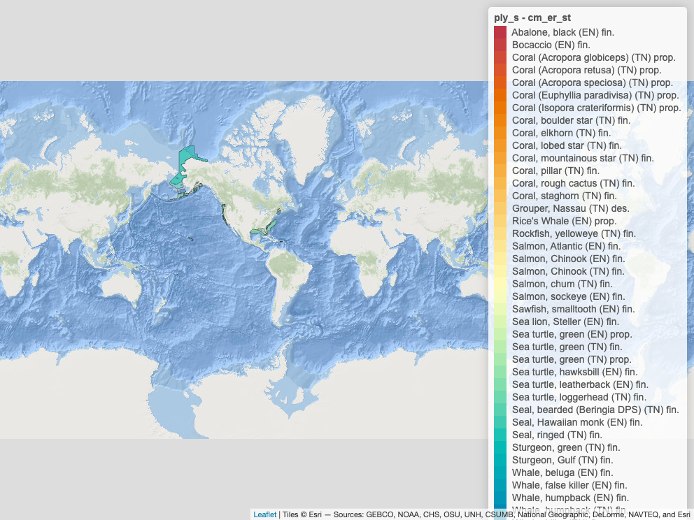
Figure 2: Polygons of Critical Habitat as a static map (Data source ply.gpkg too big (143M) for interactive display on Github-hosted notebook).
Code
ply_s |>st_drop_geometry() |>datatable()
2 Convert to MSToolkit Framework
2.1 Extinction Risk: ESA vs IUCN?
Note: ESA lists only “Endangered” or “Threatened” species, but “Threatened” is not in the IUCN RedList, so need to apply a code and score relative to others:
Extinction Risk:
CR: 1
Critically Endangered (IUCN)
EN: 0.8
Endangered (IUCN, ESA)
VU: 0.6
Vulnerable (IUCN)
TN: 0.6 Threatened (ESA)
NT: 0.4
Near Threatened (IUCN)
LC: 0.2
Least Concern (IUCN)
TODO: Check for equivalency and other issues with this comparison:
Figure 3: Rasterized polygon of Rice’s whale critical habitat as interactive map.
2.3 Default Suitability?
Originally I thought of applying a default suitability value of 50% to these binary range maps, but examples like Rice’s whale illustrate the importance of upweighting these critical habitats, so instead how about weighting by extinction risk:
Suitability:
EN: 100%
Endangered (IUCN, ESA)
TN: 80% Threatened (ESA)
The suitability value gets multiplied by the extinction risk for the species’ contribution to overall sensitivity.
ds_key <-"ch"row_dataset <-tibble(ds_key =!!ds_key,name_short ="NMFS Critical Habitat for USA, 2023-05",name_original ="National ESA Critical Habitat Geodatabase",description ="The National Marine Fisheries Service (NMFS) developed this geodatabase to standardize its Endangered Species Act (ESA) critical habitat spatial data.",citation ="",source_broad ="NMFS",source_detail ="https://www.fisheries.noaa.gov",regions ="USA",response_type ="binary",taxa_groups ="all taxa",year_pub =2023,date_obs_beg =NA,date_obs_end =NA,date_env_beg =NA,date_env_end =NA,link_info ="https://www.fisheries.noaa.gov/resource/map/national-esa-critical-habitat-mapper",link_download ="https://noaa.maps.arcgis.com/home/item.html?id=f66c1e33f91d480db7d1b1c1336223c3",link_metadata ="https://www.fisheries.noaa.gov/inport/item/65207",links_other ="https://noaa.maps.arcgis.com/apps/webappviewer/index.html?id=68d8df16b39c48fe9f60640692d0e318",spatial_res_deg =0.05,temporal_res ="static" )if (dbExistsTable(con_sdm, "dataset"))dbExecute(con_sdm, glue("DELETE FROM dataset WHERE ds_key = '{ds_key}'"))dbWriteTable(con_sdm, "dataset", row_dataset, append =TRUE)
2.6 Iterate rows: species, model, model_cell
Code
n <-nrow(d_spp_pa)tic <-Sys.time()for (i in1:n){ # i = 10 # i = 1175# for (i in 1:10){ # i = 2 sp_key <- d_spp_pa$sp_key[i] # sp_key = "ITS-Mam-180528" # sp_key = "Fis-34595" n_cells_pa <- d_spp_pa$n_cells_pa[i] toc <-Sys.time() dt <-difftime(toc, tic, units ="mins") # |> as.numeric() eta <- tic + (dt / i) * nlog_info("Processing {format(i, big.mark=',')}/{format(nrow(d_spp_pa), big.mark=',')}: {sp_key} ~ ETA: {eta}")# source(here("libs/am_functions.R"))# source(here("libs/sdm_functions.R")) r_am <-am_sp_rast(sp_key, con_am, r_hcaf) |>rotate() # [rotate() shifts cells of non-global spatRast](https://github.com/rspatial/terra/issues/1831) r_ds <-downsample_sp_rast(r_am, r_cell$depth_mean)# get species info from original database sp_info <-tbl(con_am, "spp") |>filter(sp_key ==!!sp_key) |>collect()# delete existing model mdl_seqs <-tbl(con_sdm, "model") |>filter(ds_key =="am_0.05", taxa ==!!sp_key) |>pull(mdl_seq)if (length(mdl_seqs >0)) {dbExecute(con_sdm, glue("DELETE FROM model WHERE ds_key = 'am_0.05' AND taxa = '{sp_key}'"))dbExecute(con_sdm, glue("DELETE FROM model_cell WHERE mdl_seq IN ({paste(mdl_seqs, collapse = ',')})"))dbExecute(con_sdm, glue("DELETE FROM species WHERE ds_key = 'am_0.05' AND taxa = '{sp_key}'")) }# create model for this species (one model per species for AquaMaps) d_model <-tibble(ds_key ="am_0.05",taxa = sp_key, # for AquaMaps, taxa equals sp_keytime_period ="2019",region ="Global",mdl_type ="suitability",description =glue("AquaMaps suitability for {sp_info$genus[1]} {sp_info$species[1]}, interpolated to 0.05° resolution") )dbWriteTable(con_sdm, "model", d_model, append =TRUE)# get the mdl_seq that was just created mdl_seq <-dbGetQuery(con_sdm, glue(" SELECT mdl_seq FROM model WHERE ds_key = '{d_model$ds_key}' AND taxa = '{d_model$taxa}' ORDER BY mdl_seq DESC LIMIT 1 "))$mdl_seq# determine species category sp_cat <-case_when( sp_info$class[1] =="Actinopterygii"~"fish", sp_info$class[1] =="Chondrichthyes"~"fish", sp_info$class[1] =="Mammalia"~"marine mammal", sp_info$class[1] =="Reptilia"~"sea turtle", sp_info$phylum[1] =="Mollusca"~"mollusk",# sp_info$phylum[1] == "Arthropoda" && sp_info$subphylum[1] == "Crustacea" ~ "crustacean", sp_info$phylum[1] =="Arthropoda"~"crustacean",TRUE~"other")# add species to database d_species <-tibble(ds_key ="am_0.05",taxa = sp_key,sp_key = sp_key,aphia_id =NA_integer_, # TODO: lookup from WoRMSgbif_id =NA_integer_, # TODO: lookup from GBIFitis_id =NA_integer_, # TODO: lookup from ITISscientific_name =glue("{sp_info$genus[1]} {sp_info$species[1]}"),common_name = sp_info$common_name[1],sp_cat = sp_cat)dbWriteTable(con_sdm, "species", d_species, append = T) d_mdl_cell <-as.data.frame(r_ds, cells = T, na.rm = T) |>tibble() |>mutate(mdl_seq = mdl_seq,value =as.integer(suitability) ) |>select(cell_id = cell, mdl_seq, value) |>arrange(cell_id)dbWriteTable(con_sdm, "model_cell", d_mdl_cell, append = T)}
Source Code
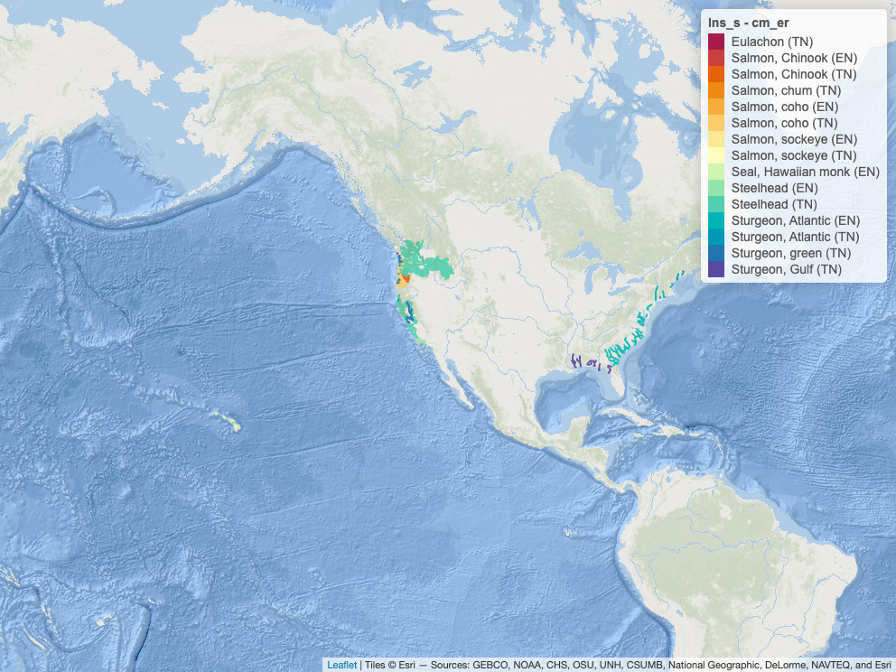
---title: "Ingest NMFS ESA Critical Habitat Geodatabase"editor_options: chunk_output_type: console---## Read NMFS ESA Critical Habitat Geodatabase- [National ESA Critical Habitat Mapper | NOAA Fisheries](https://www.fisheries.noaa.gov/resource/map/national-esa-critical-habitat-mapper) - Downloaded Geodatabase - metadata: [National ESA Critical Habitat Geodatabase | InPort](https://www.fisheries.noaa.gov/inport/item/65207) - [Threatened and Endangered Species List—Gulf of America | NOAA Fisheries](https://www.fisheries.noaa.gov/southeast/consultations/threatened-and-endangered-species-list-gulf-america)```{r setup}librarian::shelf( DBI, dplyr, DT, duckdb, fs, glue, here, knitr, leaflet, leaflet.extras2, mapview, purrr, sf, stringr, terra,quiet = T)mapviewOptions(basemaps ="Esri.OceanBasemap",vector.palette = \(n) grDevices::hcl.colors(n, palette ="Spectral") )sf_use_s2(T)is_server <-Sys.info()[["sysname"]] =="Linux"dir_private <-ifelse(is_server, "/share/private", "~/My Drive/private")iucn_tkn_txt <-glue("{dir_private}/iucnredlist.org_api_token_v4.txt")dir_data <-ifelse(is_server, "/share/data" , "~/My Drive/projects/msens/data")dir_gbif <-glue("{dir_data}/raw/gbif.org")spp_db <-glue("{dir_data}/derived/spp.duckdb")sdm_db <-glue("{dir_data}/derived/sdm.duckdb")dir_gdb <-"~/My Drive/projects/msens/data/raw/fisheries.noaa.gov"gdb <-glue("{dir_gdb}/NMFS_ESA_Critical_Habitat_20230505.gdb")lns_geo <-glue("{dir_gdb}/lns.gpkg")ply_geo <-glue("{dir_gdb}/ply.gpkg")cell_tif <-glue("{dir_data}/derived/r_bio-oracle_planarea.tif")dir_figs <-here("figs/ingest_fisheries.noaa.gov_critical-habitat")ply_png <-glue("{dir_figs}/ply.png")lns_png <-glue("{dir_figs}/lns.png")dir.create(dir_figs, showWarnings = F, recursive = T)```### Layers```{r layers}d_lyrs <-st_layers(gdb) |>tibble() |>mutate(crs =map_chr(crs, ~st_crs(.x)$input),geomtype =unlist(geomtype)) |>select(-driver) |>arrange(name)d_lyrs |>datatable()```### Lines```{r lines_map}if (!file.exists(lns_geo)){ lns <-st_read(gdb, layer ="All_critical_habitat_line_20220404", quiet = T) |>tibble() |>st_as_sf()# lns$LISTSTATUS |> table()# Endangered Threatened # 11467 48421# lns |> st_drop_geometry() |> select(LISTSTATUS, CHSTATUS) |> table()# CHSTATUS# LISTSTATUS Final# Endangered 11467# Threatened 48421 lns_s <- lns |>mutate(cm_er =case_match( LISTSTATUS,"Threatened"~glue("{COMNAME} (TN)"), # TODO: assign relative to IUCN"Endangered"~glue("{COMNAME} (EN)") ) ) |>group_by(TAXON, cm_er, SCIENAME, COMNAME, LISTSTATUS, HABTYPE) |>summarize(n =n(), .groups ="drop")st_write(lns_s, lns_geo, delete_dsn = T, quiet = T)}lns_s <-st_read(lns_geo, quiet = T)if (!file.exists(lns_png)){ m <-mapView(lns_s, alpha.regions =0.5, zcol ="cm_er")mapshot2(m, file = lns_png)}```, ".")`){#fig-lns .lightbox}```{r lines_table}lns_s |>st_drop_geometry() |>datatable()```### Polygons```{r polygons_map}if (!file.exists(ply_geo)){sf_use_s2(F) ply <-st_read(gdb, layer ="All_critical_habitat_poly_20230724", quiet = T) |>tibble() |>st_as_sf() |>st_make_valid()# ply$LISTSTATUS |> table()# Endangered Threatened # 1043 1071 # ply |> st_drop_geometry() |> select(LISTSTATUS, CHSTATUS) |> table()# CHSTATUS# LISTSTATUS Designated Final Proposed# Endangered 0 1024 19# Threatened 20 997 54 ply_s <- ply |>mutate(er =case_match( # er: extinction risk LISTSTATUS,"Threatened"~"TN","Endangered"~"EN"),st =case_match( CHSTATUS,"Designated"~"des.","Final"~"fin.","Proposed"~"prop." ),cm_er_st =glue("{COMNAME} ({er}) {st}") ) |>group_by(TAXON, cm_er_st, SCIENAME, COMNAME, LISTSTATUS, HABTYPE) |>summarize(n =n(), .groups ="drop")st_write(ply_s, ply_geo, delete_dsn = T, quiet = T)sf_use_s2(T)}ply_s <-st_read(ply_geo, quiet = T)if (!file.exists(ply_png)){ m <-mapView(ply_s, alpha.regions =0.5, zcol ="cm_er_st")mapshot2(m, file = ply_png)}```, ".")`){#fig-ply .lightbox}```{r polygons_table}ply_s |>st_drop_geometry() |>datatable()```## Convert to MSToolkit Framework### Extinction Risk: ESA vs IUCN?Note: ESA lists only "Endangered" or "Threatened" species, but "Threatened" isnot in the IUCN RedList, so need to apply a code and score relative to others:**Extinction Risk**:- `CR`: 1\ Critically Endangered (IUCN)- `EN`: 0.8\ Endangered (IUCN, **ESA**)- `VU`: 0.6\ Vulnerable (IUCN)- `TN`: **0.6** \ **Threatened** (**ESA**)- `NT`: 0.4\ Near Threatened (IUCN)- `LC`: 0.2\ Least Concern (IUCN)TODO: Check for equivalency and other issues with this comparison:- [Harris et al (2012) Conserving Imperiled Species: A Comparison of the IUCN Red List and U.S. Endangered Species Act.” Cons Lttrs](https://doi.org/10.1111/j.1755-263X.2011.00205.x)- [Threatened vs. Vulnerable - What's the Difference? | This vs. That](https://thisvsthat.io/threatened-vs-vulnerable)### Polygon to raster, eg _Balaenoptera ricei_The `terra::rasterize()` function with the 0.05° raster template provides a reasonable approximation of the original shapefile.```{r fig-ply_ricei}#| fig-cap: "Rasterized polygon of Rice's whale critical habitat as interactive map."r_cell <-rast(cell_tif)ply_ricei <- ply_s |>filter(SCIENAME =="Balaenoptera ricei")r_ricei <-rasterize( ply_ricei |>st_shift_longitude() |># [-180, 180] -> [0, 360]mutate(value =100), # TODO: default value r_cell, field ="value") |>trim()leaflet() |>addMapPane("left_pn", zIndex =0) |>addMapPane("right_pn", zIndex =0) |>addProviderTiles("Esri.OceanBasemap", group ="left_grp", layerId ="left_lyr",options =pathOptions(pane ="left_pn")) |>addProviderTiles("Esri.OceanBasemap", group ="right_grp", layerId ="right_lyr",options =pathOptions(pane ="right_pn")) |>addPolygons(data = ply_ricei,fillColor ="blue",fillOpacity =0.5,weight =1,color ="blue",group ="ply",options =pathOptions(pane ="left_pn") ) |>addRasterImage( r_ricei,colors ="red",opacity =0.8,group ="rast",options =leafletOptions(pane ="right_pn") ) |> leaflet.extras2::addSidebyside(layerId ="sidecontrols",rightId ="right_lyr",leftId ="left_lyr")```### Default Suitability?Originally I thought of applying a default suitability value of 50% to thesebinary range maps, but examples like Rice's whale illustrate the importance of upweighting these critical habitats, so instead how about weighting by extinction risk:**Suitability**:- `EN`: 100%\ Endangered (IUCN, **ESA**)- `TN`: 80%\ **Threatened** (**ESA**)The suitability value gets multiplied by the extinction risk for the species'contribution to overall sensitivity.- O'Hara et al (2017) [Aligning marine species range data to better serve science and conservation](https://journals.plos.org/plosone/article?id=10.1371/journal.pone.0175739) _PLOS One_And related:- Lee-Yaw et al (2021) [Species distribution models rarely predict the biology of real populations](https://nsojournals.onlinelibrary.wiley.com/doi/full/10.1111/ecog.05877) _Ecography_- Borgelt et al (2022) [More than half of data deficient species predicted to be threatened by extinction | Communications Biology](https://www.nature.com/articles/s42003-022-03638-9)- Moudrý & Devillers (2020) [Quality and usability challenges of global marine biodiversity databases: An example for marine mammal data](https://www.sciencedirect.com/science/article/pii/S1574954120300017?casa_token=WF_-wuk3arkAAAAA:AitcjoacX-qkxeX3ZS7WdO3rGigHo5DW4lYvGu6eELdCrY9xsd2O2b2N8hJBwY8kX1aLINU77iA) _Ecological Informatics_- O'Hara et al (2019) [Mapping status and conservation of global at-risk marine biodiversity](https://conbio.onlinelibrary.wiley.com/doi/full/10.1111/conl.12651) _Conservation Letters_- Palacio et al (2021) [A data‐driven geospatial workflow to map species distributions for conservation assessments](https://onlinelibrary.wiley.com/doi/full/10.1111/ddi.13424) _Diversity and Distributions_- Merow et al (2022) [Operationalizing expert knowledge in species' range estimates using diverse data types](https://escholarship.org/uc/item/3m7719vv) _Frontiers of Biogeography_- Ready et al (2010) [Predicting the distributions of marine organisms at the global scale](https://www.sciencedirect.com/science/article/pii/S030438000900711X?casa_token=Nrl34cYvTN4AAAAA:4_nIKkt6BcGmLZAKE-EqGO4CXPpJLaJmePucdYPQaJK3rsA8svBRDaeLYeD-1-hUbYOq3Qc1rgM) _Ecological Modelling_- Zhang et al (2025) [Differences in predictions of marine species distribution models based on expert maps and opportunistic occurrences](https://conbio.onlinelibrary.wiley.com/doi/full/10.1111/cobi.70015?casa_token=b6R7j3bt_VkAAAAA%3AUBNiiPvPiCyzF4rz8NFvu8V-AmF2VjFN7sfapmiGMI1XtU2OOItOgasjVj4a42r38fn4s7IiQ1vftnoV) _Conservation Biology_- Ferrari et al (2018) [Integrating distribution models and habitat classification maps into marine protected area planning - ScienceDirect](https://www.sciencedirect.com/science/article/pii/S0272771417310454?casa_token=TdDGGhEhrsMAAAAA:BGk07IU_j8wqaU4dg-A-JNnIAC-DCX2QL3RlhT_zwFHDkE9bHIOMSZT3MUy1XHybNR80hTdPnLQ) _Estuarine, Coastal and Shelf Science_### Line to raster, eg ...```{r lns_to_rast}``````{r evaloff}knitr::opts_chunk$set(eval = F)``````{r init_dbs}con_spp <-dbConnect(duckdb(dbdir = spp_db, read_only = T))con_sdm <-dbConnect(duckdb(dbdir = sdm_db, read_only = F))# dbListTables(con_sdm)# tbl(con_sdm, "species") |> # filter(common_name_dataset == "blue whale") |> # collect() |> # View()```### Add `dataset````{r insert_dataset_row}ds_key <-"ch"row_dataset <-tibble(ds_key =!!ds_key,name_short ="NMFS Critical Habitat for USA, 2023-05",name_original ="National ESA Critical Habitat Geodatabase",description ="The National Marine Fisheries Service (NMFS) developed this geodatabase to standardize its Endangered Species Act (ESA) critical habitat spatial data.",citation ="",source_broad ="NMFS",source_detail ="https://www.fisheries.noaa.gov",regions ="USA",response_type ="binary",taxa_groups ="all taxa",year_pub =2023,date_obs_beg =NA,date_obs_end =NA,date_env_beg =NA,date_env_end =NA,link_info ="https://www.fisheries.noaa.gov/resource/map/national-esa-critical-habitat-mapper",link_download ="https://noaa.maps.arcgis.com/home/item.html?id=f66c1e33f91d480db7d1b1c1336223c3",link_metadata ="https://www.fisheries.noaa.gov/inport/item/65207",links_other ="https://noaa.maps.arcgis.com/apps/webappviewer/index.html?id=68d8df16b39c48fe9f60640692d0e318",spatial_res_deg =0.05,temporal_res ="static" )if (dbExistsTable(con_sdm, "dataset"))dbExecute(con_sdm, glue("DELETE FROM dataset WHERE ds_key = '{ds_key}'"))dbWriteTable(con_sdm, "dataset", row_dataset, append =TRUE)```### Iterate rows: `species`, `model`, `model_cell````{r iterate_rows}n <-nrow(d_spp_pa)tic <-Sys.time()for (i in1:n){ # i = 10 # i = 1175# for (i in 1:10){ # i = 2 sp_key <- d_spp_pa$sp_key[i] # sp_key = "ITS-Mam-180528" # sp_key = "Fis-34595" n_cells_pa <- d_spp_pa$n_cells_pa[i] toc <-Sys.time() dt <-difftime(toc, tic, units ="mins") # |> as.numeric() eta <- tic + (dt / i) * nlog_info("Processing {format(i, big.mark=',')}/{format(nrow(d_spp_pa), big.mark=',')}: {sp_key} ~ ETA: {eta}")# source(here("libs/am_functions.R"))# source(here("libs/sdm_functions.R")) r_am <-am_sp_rast(sp_key, con_am, r_hcaf) |>rotate() # [rotate() shifts cells of non-global spatRast](https://github.com/rspatial/terra/issues/1831) r_ds <-downsample_sp_rast(r_am, r_cell$depth_mean)# get species info from original database sp_info <-tbl(con_am, "spp") |>filter(sp_key ==!!sp_key) |>collect()# delete existing model mdl_seqs <-tbl(con_sdm, "model") |>filter(ds_key =="am_0.05", taxa ==!!sp_key) |>pull(mdl_seq)if (length(mdl_seqs >0)) {dbExecute(con_sdm, glue("DELETE FROM model WHERE ds_key = 'am_0.05' AND taxa = '{sp_key}'"))dbExecute(con_sdm, glue("DELETE FROM model_cell WHERE mdl_seq IN ({paste(mdl_seqs, collapse = ',')})"))dbExecute(con_sdm, glue("DELETE FROM species WHERE ds_key = 'am_0.05' AND taxa = '{sp_key}'")) }# create model for this species (one model per species for AquaMaps) d_model <-tibble(ds_key ="am_0.05",taxa = sp_key, # for AquaMaps, taxa equals sp_keytime_period ="2019",region ="Global",mdl_type ="suitability",description =glue("AquaMaps suitability for {sp_info$genus[1]} {sp_info$species[1]}, interpolated to 0.05° resolution") )dbWriteTable(con_sdm, "model", d_model, append =TRUE)# get the mdl_seq that was just created mdl_seq <-dbGetQuery(con_sdm, glue(" SELECT mdl_seq FROM model WHERE ds_key = '{d_model$ds_key}' AND taxa = '{d_model$taxa}' ORDER BY mdl_seq DESC LIMIT 1 "))$mdl_seq# determine species category sp_cat <-case_when( sp_info$class[1] =="Actinopterygii"~"fish", sp_info$class[1] =="Chondrichthyes"~"fish", sp_info$class[1] =="Mammalia"~"marine mammal", sp_info$class[1] =="Reptilia"~"sea turtle", sp_info$phylum[1] =="Mollusca"~"mollusk",# sp_info$phylum[1] == "Arthropoda" && sp_info$subphylum[1] == "Crustacea" ~ "crustacean", sp_info$phylum[1] =="Arthropoda"~"crustacean",TRUE~"other")# add species to database d_species <-tibble(ds_key ="am_0.05",taxa = sp_key,sp_key = sp_key,aphia_id =NA_integer_, # TODO: lookup from WoRMSgbif_id =NA_integer_, # TODO: lookup from GBIFitis_id =NA_integer_, # TODO: lookup from ITISscientific_name =glue("{sp_info$genus[1]} {sp_info$species[1]}"),common_name = sp_info$common_name[1],sp_cat = sp_cat)dbWriteTable(con_sdm, "species", d_species, append = T) d_mdl_cell <-as.data.frame(r_ds, cells = T, na.rm = T) |>tibble() |>mutate(mdl_seq = mdl_seq,value =as.integer(suitability) ) |>select(cell_id = cell, mdl_seq, value) |>arrange(cell_id)dbWriteTable(con_sdm, "model_cell", d_mdl_cell, append = T)}```